Learning the Generator: PINN-MMST Dynamics

A trajectory contains many correlated coordinates, momenta, mapping variables, and observables, but they are all generated by one Hamiltonian. This suggests a useful hierarchy for machine learning: learn the potential or Hamiltonian that generates the dynamics instead of fitting every downstream variable independently. The idea connects machine-learned potential energy surfaces, physics-informed neural networks, and MMST mapping dynamics.

From Trajectories to Generators

For a classical Hamiltonian system with phase-space state \(\mathbf{x}=(\mathbf q,\mathbf p)\), the equations of motion are

\dot{\mathbf x}=\mathbf J\nabla_{\mathbf x}H(\mathbf x).

A purely data-driven network learns a discrete flow map,

\mathbf x_{n+1}=\Phi_{\theta,\Delta t}(\mathbf x_n),

whereas a physics-informed model learns an upstream object such as \(H_\theta\), \(V_\theta\), or the corresponding force field and lets the known equations generate the trajectory. The latter restricts the hypothesis space: position and momentum updates cannot vary independently, and the same learned potential controls every coupled degree of freedom.

The Classical ML-MD Analogy

Machine-learned molecular dynamics normally predicts a Born-Oppenheimer potential energy surface rather than the next atomic configuration directly:

\mathbf R\xrightarrow{\mathrm{MLPES}}E_\theta(\mathbf R),\qquad \mathbf F_I=-\frac{\partial E_\theta}{\partial\mathbf R_I}.

Newton's equations and an MD integrator then produce \((\mathbf R(t),\mathbf P(t))\). This is not usually called a PINN in the narrow sense, because the model is commonly trained by supervised energy and force labels rather than by a differential-equation residual. It nevertheless embodies the same broad principle: machine learning supplies the unknown generator, while established physics supplies the propagation.

The analogy with density-functional theory is conceptual rather than literal. DFT replaces the many-electron wavefunction with a more compact basic variable, the density, under the assumptions of the Hohenberg-Kohn framework. MLPES and Hamiltonian learning similarly seek a compact upstream object from which many correlated outputs follow. In ML-MD the learned quantity is normally the effective Born-Oppenheimer energy, not the known bare electron-nuclear external potential.

MMST as a Matrix-Valued MLPES

For \(F\) electronic states, MMST introduces electronic mapping variables \((q_j,p_j)\) and couples them to nuclear coordinates \((\mathbf R,\mathbf P)\). A primitive real-diabatic MMST Hamiltonian is

H_{\mathrm{MMST}}= \frac{\mathbf P^2}{2M}+ \frac12\sum_{jk}V_{jk}(\mathbf R) \left(q_jq_k+p_jp_k-2\gamma\delta_{jk}\right).

The multi-state analogue of an MLPES is therefore a matrix-valued model,

\mathbf R\longrightarrow\mathbf V_\theta(\mathbf R)=\{V_{jk,\theta}(\mathbf R)\}.

Once this matrix and its nuclear gradients are known, Hamilton's equations determine all variables:

\dot{\mathbf q}=\mathbf V(\mathbf R)\mathbf p, \qquad \dot{\mathbf p}=-\mathbf V(\mathbf R)\mathbf q,

\dot{\mathbf R}=\frac{\mathbf P}{M}, \qquad \dot{\mathbf P}=-\frac12\sum_{jk}\nabla_{\mathbf R}V_{jk} \left(q_jq_k+p_jp_k-2\gamma\delta_{jk}\right).

This structure also explains a useful invariant. For a real symmetric \(\mathbf V\),

\frac{d}{dt}\left(\mathbf q^\mathrm{T}\mathbf q+\mathbf p^\mathrm{T}\mathbf p\right) =2\mathbf q^\mathrm{T}\mathbf V\mathbf p-2\mathbf p^\mathrm{T}\mathbf V\mathbf q=0.

A direct state-to-state network has no reason to preserve this mapping radius. A physics-informed propagator inherits the continuous MMST coupling structure, although exact numerical conservation still depends on the integrator and architecture.

What the PINN Learns

The PINN studied here predicts the potential-related quantities and embeds them inside a differentiable RK4 MMST step. The data-driven comparator predicts a normalized one-step phase-space increment directly. Their roles can be summarized as follows.

Model	Learned object	Fixed structure	Expected trade-off
DD-FCN	Discrete map \(\mathbf x_n\mapsto\mathbf x_{n+1}\)	Only the residual form and training data	Cheap steps, but rollout errors can violate coupled phase-space relations
PINN-FCN	Potential/gradient maps and selected scalars	MMST equations and RK4 stages	More expensive steps, but a smaller and physically structured hypothesis space

A stronger future implementation would predict only a symmetric \(\mathbf V_\theta(\mathbf R)\) and obtain every gradient through automatic differentiation. The present benchmark follows the paper more closely by representing potential and gradient maps separately, so potential-force consistency is encouraged through trajectory training rather than guaranteed by construction.

A Reproducible Small-N Check

The numerical check uses the Ohmic spin-boson parameters of Zeng and Sun but reduces the bath from \(N=100\) to \(N=4\). It uses two sigmoid hidden layers of 256 units, 256 training trajectories of 500 steps, 64 validation trajectories, and two independent 256-trajectory test batches. This is a constrained implementation smoke test, not a reproduction of the published \(N=100\) figures. Mapping-sphere projection and an explicit mapping constraint were added as numerical stabilizers and are not claimed to be part of the reported paper protocol.

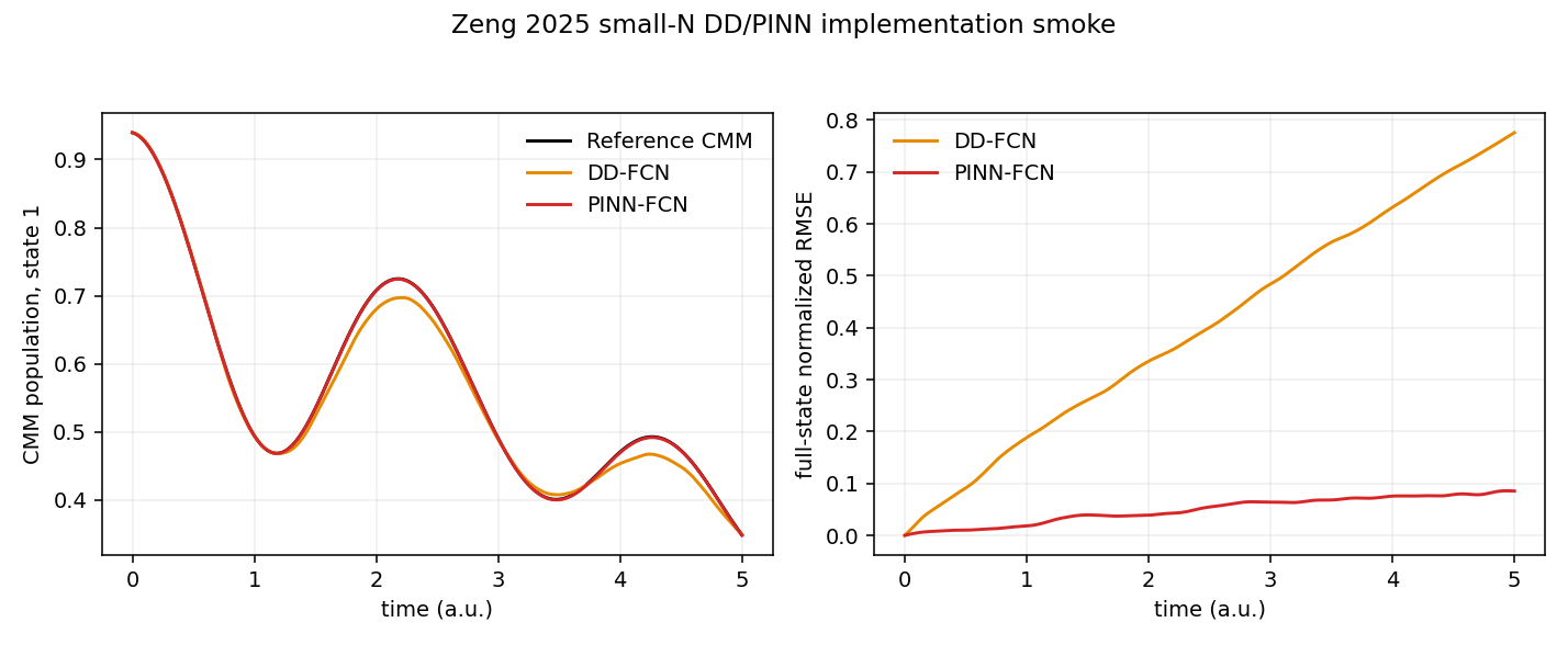
Reference CMM, data-driven FCN, and physics-informed FCN population and rollout-error comparison — Small-\(N\) CMM benchmark over 0 to 5 reduced time units. Left: state-1 ensemble population; black is reference CMM, orange is DD-FCN, and red is PINN-FCN. Right: full-state normalized RMSE for recursive rollout; orange is DD-FCN and red is PINN-FCN. No smoothing was applied. The PINN population remains visually coincident with the reference while the unrestricted DD rollout accumulates a larger phase-space error.

Diagnostic	DD-FCN	PINN-FCN
Population RMSE	0.013303	0.000563
Maximum population error	0.028676	0.001201
Maximum full-state rollout NRMSE	0.775512	0.085812
Mapping-radius maximum drift	Not used as an acceptance claim	\(3.89\times10^{-6}\)

The reference trajectory passed a time-step-halving population check with a maximum difference of \(1.75\times10^{-6}\), and its maximum relative energy drift was \(3.62\times10^{-5}\). Both independent test batches and predeclared finite-value, monotonic-grid, roughness, spike, and endpoint-artifact checks passed. In this particular benchmark, the PINN population RMSE is about 24 times smaller than the DD-FCN value. This factor is an empirical result for this configuration, not a general theorem about PINNs.

Accuracy Is Not Acceleration

The analytic spin-boson reference is cheaper than a neural network, so this benchmark demonstrates structured accuracy rather than wall-time acceleration. A meaningful speedup appears only when the learned potential replaces an expensive electronic-structure evaluation. For a production calculation, the relevant metric is time to a fixed observable accuracy, not inference time alone:

S_{\mathrm{effective}}= \frac{\min T_{\mathrm{reference}}\;\text{subject to error}<\varepsilon} {\min T_{\mathrm{PINN}}\;\text{subject to error}<\varepsilon}.

Training and reference-data generation must be amortized. If \(T_\mathrm{upfront}\) is the data, training, and validation cost, the break-even number of production trajectories is

N_{\mathrm{break-even}}= \frac{T_\mathrm{upfront}} {T_\mathrm{ref,traj}-T_\mathrm{PINN,traj}}.

A defensible benchmark should report potential-and-gradient evaluation time, complete trajectory throughput, time-step convergence, ensemble confidence intervals, and total time to a target population error. A DD model may be faster per step because it needs only one forward pass, while a PINN may win at fixed long-time accuracy because its rollout remains physically coherent.

Beyond Toy Models

MMST-derived dynamics are not limited to toy models. On-the-fly SQC/MMST has been applied to methaniminium and azomethane, while recent ab initio spin-mapping calculations have treated ethylene, fulvene, methyliminium, and 1,2-dithiane with CASSCF electronic structure. The PySurf implementation now provides a common framework for several quasiclassical mapping schemes. Nevertheless, the specific PINN-MMST literature considered here remains at the model-Hamiltonian stage.

The difficult transition is not merely increasing the number of bath modes. A realistic ML-MMST model must handle smooth multi-state energies, gradients, state overlaps, phase conventions, quasi-diabatic transformations, and uncertainty near conical intersections. It must also separate surrogate error from the intrinsic approximations of MMST, such as population leakage, detailed-balance errors, and sensitivity to zero-point parameters or windowing.

A practical development path is therefore

\text{spin-boson}\rightarrow \text{multi-mode LVC}\rightarrow \text{precomputed molecular surfaces}\rightarrow \text{on-the-fly or ML Hamiltonian MMST}.

Code

run_reproduction.py generates the dataset, trains DD-FCN and PINN-FCN models with restartable checkpoints, performs recursive rollouts, and writes the physical and curve-quality audits.
config_smalln.json freezes the model parameters, training protocol, stabilizers, scope limits, and all acceptance thresholds before evaluation.
curve_quality.py provides the machine-readable smoothness, spike, endpoint, and monotonic-grid diagnostics used by the acceptance audit.

python assets/code/mmst-pinn/run_reproduction.py \
  --config assets/code/mmst-pinn/config_smalln.json \
  --output scratch/mmst-pinn-smalln

The run requires Python, PyTorch, NumPy, SciPy, pandas, Matplotlib, and scikit-learn. A CUDA device is recommended for the published 300-epoch configuration. Generated checkpoints and trajectory archives should remain local rather than being committed to the website.

References

H. Zeng and X. Sun, "Data-Driven Versus Physics-Informed Neural Networks for Nonadiabatic Semiclassical Mapping Dynamics," Communications in Computational Chemistry 7, 217-225 (2025), doi:10.4208/cicc.2025.152.01.
K. Lin, J. Peng, C. Xu, F. L. Gu, and Z. Lan, "Trajectory Propagation of Symmetrical Quasi-classical Dynamics with Meyer-Miller Mapping Hamiltonian Using Machine Learning," Journal of Physical Chemistry Letters 13, 11678-11688 (2022), doi:10.1021/acs.jpclett.2c02159.
D. Hu, Y. Xie, J. Peng, and Z. Lan, "On-the-Fly Symmetrical Quasi-Classical Dynamics with Meyer-Miller Mapping Hamiltonian for the Treatment of Nonadiabatic Dynamics at Conical Intersections," Journal of Chemical Theory and Computation 17, 3267-3279 (2021), doi:10.1021/acs.jctc.0c01249.
B. M. Weight, A. Mandal, D. Hu, and P. Huo, "Ab Initio Spin-Mapping Non-Adiabatic Dynamics Simulations of Photochemistry," Journal of Chemical Physics 162, 084105 (2025), doi:10.1063/5.0248950.
D. Picconi et al., "Implementation of Quasiclassical Mapping Approaches for Nonadiabatic Molecular Dynamics in the PySurf Package," Physical Chemistry Chemical Physics 27, 19105-19122 (2025), doi:10.1039/D5CP01194A.