Reaction-Rate Methods · Sequel
From Reactants or the Dividing Surface? An N=1 Equivalence Test
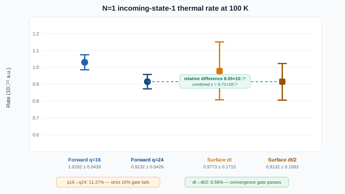
There are two apparently different ways to initialize a nonadiabatic reaction-rate trajectory. One launches a pure incoming electronic state in the reactant asymptote. The other starts directly at the interaction-region dividing surface and reconstructs the missing electronic history backward in time. At one bead, after converging the energy quadrature and the trajectory time step, the two calculations give (9.132066 imes10^{-12}) and (9.132144 imes10^{-12}) a.u. Their relative difference is (8.55 imes10^{-6}). For this rate observable, they are the same calculation expressed through two sampling measures.
This is a sequel to Comparing Trajectory Dynamics with Kubo Flux-Side Correlations. The previous article explained how a reactant-launched, barrier-conditioned trajectory ensemble can be compared with a Kubo flux-side correlation. The unresolved question was whether Tully's much more elaborate dividing-surface initialization estimates that same object. Here the question is isolated at (N=1), where ring-polymer complications disappear.
The Question Being Tested
The comparison is not between CSSH and RPSH as complete methods. It freezes the same one-dimensional two-state Hamiltonian, the same fewest-switches hopping rule, the same frustrated-hop policy, the same electronic propagator, and the same asymptotic product indicator. Only the sampling representation of the thermal rate changes:
| Estimator | Initial point | Electronic condition | Rare-event treatment |
|---|---|---|---|
| Forward | Reactant asymptote | Pure incoming state (a) | Boltzmann energy integral |
| Surface | (R=R^ddagger) | Reconstructed from a backward history | TST prefactor, likelihood ratio, and crossing correction |
Why \(N=1\) Isolates Initialization
For \(N\) beads, the free ring-polymer part of the nuclear Hamiltonian is
At \(N=1\), cyclic closure gives \(R_1-R_1=0\), so the spring term vanishes and the centroid is the physical coordinate: \(\bar R=R_1\). The two electronic approximations then collapse as well:
The active-surface force, momentum, NAC drive, and hopping probability are therefore those of the same single-copy FSSH trajectory. No bead average or centroid replacement survives. Any discrepancy left at \(N=1\) must come from the way paths are initialized and counted, from the backward-history likelihood ratio, or from numerical quadrature, time step, and statistics.
Why Both Estimators Target One Flux-Side Rate
Step 1: write the reactant-side positive-flux ensemble
Put a dividing surface \(R_A\) in the reactant asymptote, where the two electronic states are degenerate and the NAC has vanished. Let \(\mathcal P_{ab}(P)\) be the probability—averaged over the stochastic FSSH decisions—that a trajectory launched with \(P>0\) in the pure electronic state \(a\) reaches products in state \(b\). The classical mixed quantum–classical flux-side rate per reactant length is
With the asymptotic energy zero \(V_a(R_A)=0\), the two degenerate reactant electronic states give
Now set \(E=P^2/(2M)\). Because \(dE=(P/M)dP\), the velocity factor is exactly the Jacobian of the momentum-to-energy transformation. Using \(d(\beta E)=\beta\,dE\) gives
The factor \(1/2\) is therefore not fitted; it comes from the electronic degeneracy in \(Q_A\). If transmission is classically impossible below a threshold \(\Delta\), write \(E=\Delta+x/\beta\). Then \(e^{-\beta E}=e^{-\beta\Delta}e^{-x}\), so
which is evaluated deterministically by Gauss–Laguerre quadrature. This is the energy-integrated analogue of sampling an exponentially distributed above-barrier excess energy.
Step 2: insert every positive crossing without changing a path's weight
Consider one complete reactive path \(X\), and let \(n_+[X]\) be its number of positive-direction crossings of an internal surface \(R^\ddagger\). The delta-function identity
follows from \(\delta[f(t)]=\sum_j\delta(t-t_j)/|f'(t_j)|\): every positive crossing contributes one. Thus, for the reactive-path indicator \(\chi_{ab}[X]\),
Inserting this identity into the reactant-launched path integral changes neither the path nor its weight. It only re-indexes the ensemble by positive crossing events. Assuming a stationary thermal path measure, time translation moves the sampled crossing to \(t=0\), producing the familiar internal-surface factorization
A trajectory sampled directly at \(R^\ddagger\) sees the same physical path once for every positive crossing. The factor \(1/n_+\) is therefore not a dynamical approximation; it is the multiplicity correction that makes the event-indexed ensemble count each complete reactive path once:
Step 3: recover the incoming electronic boundary condition
A local active state \(i\) at \(R^\ddagger\) does not identify the reactant incoming state \(a\). The electronic amplitudes at the surface are therefore obtained by inverting the unitary electronic propagator subject to
The auxiliary backward algorithm draws a hop/no-hop history \(H=(e_1,\ldots,e_L)\) from a proposal distribution \(Q(H)\). The corresponding physical forward FSSH history has probability \(P(H\mid a)\). If the proposal covers the target support, \(Q(H)>0\) whenever \(P(H\mid a)>0\), the Radon–Nikodym derivative is
and unbiased reweighting follows by direct summation:
This is why assigning an electronic Boltzmann population locally at the dividing surface would answer a different question: it would not enforce the pure incoming boundary condition and would not reproduce the forward FSSH path measure.
Step 4: convert half-Maxwell sampling into positive flux
The code samples the canonical momentum conditioned only on \(P>0\),
rather than sampling the already flux-weighted density proportional to \(P e^{-\beta P^2/(2M)}\). Consequently, the velocity \(P/M\) must appear once in both the reactive numerator and the normalization denominator. The implemented transmission coefficient is
Multiplying this ratio by \(k_i^{\mathrm{TST}}\) restores the Boltzmann penalty for reaching surface \(i\). Summing over all dividing-surface states \(i\), incoming states \(a\), and final states \(b\) restores the complete electronic trace. Under the same Hamiltonian and FSSH rules, correct history support and likelihood ratios, crossing correction, stationary thermal measure, and converged numerical limits,
The equality is a change of sampling measure, not a claim that the two generated microscopic histories are identical trajectory by trajectory.
What the Algorithms Actually Do
Reactant-launched estimator
The forward implementation constructs the quadrature energies, runs an energy-resolved FSSH scattering ensemble for each incoming state, and contracts the transmission probabilities with the thermal weights:
beta = 1.0 / (kB * temperature)
nodes, weights = np.polynomial.laguerre.laggauss(q)
energies = energy_shift + nodes / beta
weights = np.exp(-beta * energy_shift) * weights

for energy_index, energy in enumerate(energies):
    estimate = run_energy_resolved_classical_fssh(
        total_energy=energy,
        incoming_state=incoming,
        x_start=-3.0,
        reactant_boundary=-3.05,
        product_boundary=2.0,
        frustrated_hop_policy="keep",
    )
    probability[energy_index] = estimate.transmitted / estimate.ntraj

free_flux = 0.5 / np.sqrt(2.0 * np.pi * mass * beta)
rate = free_flux * np.dot(weights, probability)
Dividing-surface estimator
The surface sampler first draws canonical momenta conditioned on positive centroid momentum. It then reconstructs a backward electronic history, launches the physical forward path, and divides a reactive contribution by its positive crossing multiplicity:
momenta = rng.normal(0.0, np.sqrt(mass * nbeads / beta), nbeads)
pbar = np.mean(momenta)
if pbar < 0.0:
    momenta -= 2.0 * pbar          # half-Maxwell centroid

f = trial_hop_probabilities(coupling, active, dt)
g = physical_forward_fssh_probabilities(history, active, dt)
step_factor = g[physical_target] / f[proposal_target]
W = np.prod(step_factors)

nplus = count_forward_crossings(path, dividing_surface)
corrected = W / nplus if reactive and nplus > 0 else 0.0

flux = pbar / mass
kappa = np.mean(flux * corrected) / np.mean(flux)
rate = k_tst * kappa
The dividing-surface electronic amplitudes are not assigned from a local Boltzmann population. They are obtained by inverting the unitary electronic propagation so that the backward endpoint satisfies the pure incoming condition. Hop and no-hop likelihood factors then convert the artificial backward proposal into the physical forward history measure.
The Remaining Theoretical Gap: Finite-Step Reversal
The change-of-measure identity is exact only if the proposal covers the physical path support and the reverse mapping is correct. The electronic event tree was verified to normalize for one- and two-step histories. A full discrete nuclear path is subtler: the backward algorithm propagates on a surface and then proposes a hop, whereas its literal reverse is a hop followed by propagation. These orderings become the same as (Delta t\to0), but they are not an exact finite-step theorem.
This is why simply adding more trajectories would have been a poor test. The calculation first had to close two independent systematic errors: the forward energy quadrature and the surface-trajectory time step.
Pre-Registered N=1 Convergence Test
The test used the 100 K, one-dimensional, two-state reaction model of Shushkov, Li, and Tully. Incoming state 1 was selected because an earlier low-statistics calculation showed the largest apparent disagreement there. All other choices were frozen: midpoint-exponential electronic propagation, one nuclear substep, frustrated-hop policy keep, the physical_forward_bijective history convention, and boundaries (-3.05/2.0) bohr.
| Systematic check | Levels | Independent sampling | Gate |
|---|---|---|---|
| Forward energy integral | (q=16,24) | 3 replicates, 50 trajectories per energy | Combined (2\sigma) and ≤10% relative change |
| Surface time step | 0.0036, 0.0018 fs | 3 replicates × 16 blocks × 25 trajectories | Combined (2\sigma) and ≤10% relative change |
| Estimator equivalence | (q=24) versus (Delta t/2) | Independent estimators | Combined (2\sigma) |
In total, 216 compact result blocks contained 8,400 trajectories. Every task completed with empty standard error logs. A strict validator checked the temperature, bead count, incoming state, quadrature and seed grids, finite values, transmission counts, hop budgets, crossing histograms, and effective sample sizes. The minimum nonzero contribution ESS fraction was 4%.
Results
| Comparison | First rate (a.u.) | Second rate (a.u.) | Relative difference | (z) | Decision |
|---|---|---|---|---|---|
| Forward (q=16\to24) | ((1.029152\pm0.043851)\times10^{-11}) | ((0.913207\pm0.042551)\times10^{-11}) | 11.27% | -1.898 | Strict 10% gate fails |
| Surface (Delta t\to\Delta t/2) | ((0.977350\pm0.171540)\times10^{-11}) | ((0.913214\pm0.108330)\times10^{-11}) | 6.56% | -0.316 | Pass |
| (q=24) forward vs. (Delta t/2) surface | ((0.913207\pm0.042551)\times10^{-11}) | ((0.913214\pm0.108330)\times10^{-11}) | (8.55\times10^{-6}) | (6.71\times10^{-5}) | Pass |
The Plain-Language Conclusion
At (N=1), reactant launch and dividing-surface history reconstruction give the same thermal rate once the two numerical representations are sufficiently resolved. The elaborate surface construction is not introducing a persistent 30% bias. An earlier calculation had reported a surface/forward ratio of 0.681 for incoming state 1, but that comparison used only eight energy nodes and much weaker surface statistics. The discrepancy disappears when both error budgets are resolved.
There is nevertheless one deliberate qualification. The overall pre-registered gate is still recorded as not passed, because the forward result changes by 11.27% between (q=16) and (q=24), just beyond the 10% limit. The near-perfect (q=24)-versus-half-step agreement is extremely strong positive evidence, but it does not justify changing a convergence rule after seeing the result.
The honest statement is therefore:
What This Does—and Does Not—Establish
- Established numerically: the two initialization schemes are consistent estimators of the same (N=1) incoming-state-resolved thermal rate.
- Diagnosed: the former 32% discrepancy was not evidence of a stable missing-history weight; insufficient energy resolution and finite statistics were enough to create it.
- Not established: equality of the full crossing-conditioned electronic distributions, phases, or individual microscopic paths.
- Not generalized: the result says nothing about the validity of bead-averaged NACs at (N>1). That is a separate BA approximation problem.
- Still open: a (q=32) or (q=40) deterministic check would close the strict quadrature gate more cleanly than adding more trajectories at the same quadrature order.
Executable Algorithm Core
- n1_flux_side_equivalence_core.py contains executable, self-checking implementations of the shifted Gauss–Laguerre forward estimator, positive-centroid canonical momentum sampling, path-likelihood reweighting, the (1/n_+) surface estimator, and the combined-(\sigma) convergence test.
- cssh_rate_algorithm.py supplies the complementary trajectory-level machinery used in the preceding article: electronic propagation, fewest-switches trial probabilities, accepted hops, frustrated hops, and conditional thermal-rate estimation.
References
- Shushkov, Li, and Tully, “Ring polymer molecular dynamics with surface hopping,” J. Chem. Phys. 137, 22A549 (2012), doi:10.1063/1.4766449.
- Tully, “Molecular dynamics with electronic transitions,” J. Chem. Phys. 93, 1061 (1990).
- Comparing Trajectory Dynamics with Kubo Flux-Side Correlations, the preceding article in this sequence.