HefeiNAMD Series - Part III
The EPC Route to Carrier Dynamics
Part II admitted finite-wavevector nuclear motion by enlarging the simulation cell, then obtained nonadiabatic coupling from electronic wavefunctions along the trajectory. The electron-phonon coupling (EPC) route builds the time-dependent electronic Hamiltonian from a different starting point: reference Bloch states, their linear response to lattice displacements, and phonon coordinates that evolve in time.
The central chain is reference electronic structure + phonon modes + EPC matrix elements + a nuclear path → electronic Hamiltonian → carrier dynamics. A phonon dispersion alone supplies only part of this information. We will derive the matrix construction, identify where the trajectory enters, and separate the underlying idea from choices made by the public HefeiNAMD-EPC implementation.
Practical FAQ: choosing real-space or EPC dynamics, comparing Hamiltonians and hopping rules, and using finite-temperature phonons. Appendix A derives the hopping probabilities in fixed diabatic and moving adiabatic bases.
1. Keep the reference electronic basis fixed
Choose a reference geometry \(\mathbf R_0\). Its Kohn-Sham (KS) Hamiltonian defines the Bloch states and energies
The basis states remain those of \(\mathbf R_0\), even when the nuclei move. Consequently their time derivatives vanish. The physical electronic Hamiltonian at a displaced geometry is generally not diagonal in this basis:
This is a fixed reference Bloch representation. It has the practical character of a diabatic representation, but choosing it does not establish a globally complete, strictly diabatic finite band manifold. The retained states must still cover the dynamics of interest. This representation is the starting point of Zheng et al.'s momentum-space formulation, Eqs. (5)–(9).
2. Expand the electronic Hamiltonian in displacement
Let \(u_{l\kappa a}\) be the displacement of atom \(\kappa\), in primitive cell \(l\), along Cartesian direction \(a\). The leading change in the electronic Hamiltonian is
The derivative describes how the electrons respond to moving an atom. In a self-consistent KS calculation, it includes the induced change in electronic density and potential, not merely the derivative of a bare ionic potential. Keeping this term defines linear EPC. Computing it once lets us assemble approximate Hamiltonians for many displacements without solving a fresh electronic eigenproblem at every time.
This approximation is distinct from the harmonic approximation to the nuclear potential energy \(U\):
Here \(I,J\) collect atomic and Cartesian indices, and the linear nuclear-energy term vanishes at equilibrium. Linear EPC truncates the electronic operator after first order. Harmonic nuclear dynamics truncates the nuclear potential energy after second order. One may use a nonharmonic trajectory with linear EPC, but doing so does not restore the electronic terms that were omitted.
3. Phonons organize the atomic displacements
Consider a Born-von Kármán periodic crystal containing \(N_p\) primitive cells. Normalize the dimensionless phonon eigenvectors by
Using mass-weighted normal coordinates \(Q_{\mathbf q\nu}\), expand the displacement as
\(\mathbf R_l\) is the equilibrium lattice vector, \(M_\kappa\) is the atomic mass, \(\mathbf q\) is the phonon wavevector, and \(\nu\) labels its branch. The eigenvector specifies which atoms move and in which directions; \(Q(t)\) specifies how far along that pattern the system has moved. The frequency \(\omega_{\mathbf q\nu}\) supplies its harmonic time scale.
Real atomic displacements require matched opposite-wavevector modes. In a consistent phase convention,
They cannot be sampled as two unrelated real vibrations. Independent real sine and cosine modes provide one convenient way to enforce this condition. A phonon dispersion gives the frequencies; it does not specify the normal coordinates, their initial amplitudes, or their phases.
4. EPC matrix elements measure the electronic response to a mode
Insert the displacement expansion into the linear electronic Hamiltonian. Define the mode derivative operator
The matrix element of this operator asks a concrete question: how strongly does this displacement pattern mix two reference electronic states? Translating the crystal produces a lattice phase sum
Thus a mode with wavevector \(\mathbf q\) connects \(\mathbf k\) to \(\mathbf k+\mathbf q\), modulo a reciprocal lattice vector \(\mathbf G\). For nonzero \(\mathbf q\), this perturbation carries finite crystal momentum, unlike the translation-preserving path in Part I. Other symmetries may still make an allowed matrix element vanish.
For each stable, nonzero-frequency mode define a mass-weighted zero-point scale and an energy-valued EPC matrix element:
The Bloch states here are normalized over the full periodic crystal. With mass-weighted \(Q\), both \(Q\) and \(\ell\) have units of square-root mass times length; \(Q/\ell\) is dimensionless and \(g\) has units of energy. Some conventions introduce a reference mass and a length-valued normal coordinate instead. The product \(gQ/\ell\) must remain consistent when changing conventions.
The full-operator definition also accommodates nonlocal terms. For a local potential, extracting its Bloch phase yields the usual primitive-cell matrix element between cell-periodic electronic functions. The EPW theory documentation gives that standard convention and the self-consistent perturbation construction. Frequencies and polarization vectors alone cannot supply \(g\): they describe the lattice, while \(g\) also depends on the electronic states and their response.
5. Multiply each response by its actual displacement
The linear EPC Hamiltonian in the fixed reference basis is now
The three ingredients have separate jobs. \(g\) measures the electronic sensitivity to a mode; \(Q(t)/\ell\) measures its instantaneous displacement; the momentum condition selects the electronic state pairs it can connect. The reference energies provide the unperturbed spectrum. Even a large \(g\) produces no instantaneous linear perturbation when that coordinate is zero. A nonzero coordinate can also shift diagonal energies, particularly through q = 0 contributions.
The complex phases of \(g\), the electronic states, and the phonon eigenvectors must be consistent. A table of \(|g|^2\), adequate for some rate formulas, does not generally contain enough phase information to reconstruct this Hamiltonian. Opposite-q matching and the Hermitian electronic response must yield \(H(t)=H^\dagger(t)\). \(N_p\) belongs to the normalization volume and cannot be changed as an arbitrary coupling-strength parameter.
Dense k/q grids can be generated through primitive-cell perturbation calculations and interpolation. They represent many spatial wavelengths without explicitly running a molecular-dynamics trajectory in an equally large real-space cell. The wavelengths have not disappeared: they are encoded in the q grid and mode coordinates. This reduces one source of cost, while matrix-element storage, band truncation, and k/q convergence remain.
6. The Hamiltonian still needs a nuclear path
For an independent, mass-weighted real harmonic mode, let \(P=\dot Q\) and write
The frequency does not determine \(Q_0\) or \(P_0\). An initial ensemble or a specified preparation must supply them. In a quantum thermal harmonic oscillator, with \(\beta=1/(k_BT)\), the coordinate variance is
This identifies a thermal fluctuation scale, including a zero-point term. It does not uniquely prescribe a collection of real-time trajectories or make a classical coordinate into a quantum operator.
For example, Gaussian Wigner sampling with this coordinate variance, momentum variance \(\hbar\omega(2n+1)/2\), and zero coordinate-momentum covariance reproduces the independent harmonic mode's symmetrized linear-coordinate correlation under harmonic propagation. The ordinary ordered quantum correlation additionally has an imaginary commutator contribution. Keeping a zero-point variance alone therefore does not establish quantum absorption/emission asymmetry or detailed balance. This example is an ensemble choice, not a description of the default code sampler.
In the inspected public source, EPCTYPE=1 initializes two equal real factors \(\sqrt{n+1/2}\) and advances their positive- and negative-frequency phases. For matched frequencies their sum corresponds to
This branch does not randomly sample the initial phonon phases. Different initial-time offsets select different segments of the prescribed oscillations. The Bose factor changes the driving amplitude; it does not by itself renormalize the input harmonic frequencies into a finite-temperature anharmonic dispersion.
A second conceptual route is to obtain \(\mathbf u(t)\) from an atomic trajectory and project it onto the reference modes:
This can carry nonharmonic time dependence, provided the trajectory contains the required wavelengths. A small primitive-cell trajectory still cannot generate missing finite-q modes by projection. The repository has an EPCTYPE=2 decomposition routine, but the inspected active propagation path does not establish a complete connection from its projected-coordinate array to the Hamiltonian driver. That interface needs verification before being treated as a working alternative. Rigid zero-frequency translations must be handled separately, and unstable imaginary-frequency modes cannot be inserted into a stable thermal harmonic-oscillator prescription.
7. Propagate the electrons, then specify the hopping approximation
With \(a,b\) denoting band-and-k pairs, the fixed-basis coefficient equation is simply
Compare this with the instantaneous adiabatic representation of Part II, whose coefficient propagation matrix is \(\epsilon_\alpha(t)\delta_{\alpha\beta}-i\hbar d_{\alpha\beta}(t)\). There the off-diagonal term arises from the moving basis. Here the basis is fixed and the displaced physical Hamiltonian has off-diagonal elements. Energy-valued \(g\) is not a numerical substitute for inverse-time NAC \(d\).
For complete representations of the same model and path, a time-dependent unitary basis transformation relates these two descriptions, including the moving-basis term. Actual calculations also differ through displacement truncation, nuclear paths, band windows, and hopping choices. Merely changing representation does not make those approximations equivalent.
Electronic propagation alone determines coherent amplitudes. Its outward population current is
A stochastic active-state scheme is an additional construction; Part II explains the fewest-switches surface-hopping (FSSH) idea. In this EPC source, electronic propagation uses the time-dependent matrix, while the switching routine also uses precomputed, broadened scattering weights built from squared EPC amplitudes, occupations, and energy matching, with a thermal acceptance factor. These weights are neither \(H_{ab}(t)\) itself nor a consequence forced by the basis transformation. The switching model must be assessed separately from the Hamiltonian construction.
The classical-path approximation (CPA) is another independent choice: the nuclei or mode coordinates follow a prescribed path without responding dynamically to the selected electronic excitation. It is not defined by the use of a fixed basis. In the inspected branch, accumulated phonon-excitation counts are separate from the coordinates driving \(H(t)\); reporting such counts does not establish feedback into the next nuclear step.
8. Hands-on: the official graphene tutorial
The authors' June 2024 training slides, pp. 21–35, turn the construction above into a concrete question: how does an electron initially about 1 eV above the graphene band reference lose energy, and which phonon branches receive it? This section follows that example and compares an existing run with the original figures on slide 34. It uses the full tutorial grid and inputs, rather than a reduced demonstration.
8.1 Start from the supplied first-principles data
The complete upstream chain is a Quantum ESPRESSO electronic calculation, density-functional perturbation theory for phonons, Wannierization, and qe2pert.x. The resulting graphene_epr.h5 contains the information needed for subsequent interpolation. For this run, that stage was reused from Perturbo's official example outputs, under example05-graphene-2d/qe2pert/References. The corresponding SCF, NSCF, Wannier, and pseudopotential inputs were checked against the NAMD example; phonon inputs differ only in task splitting. No new SCF or DFPT calculation was performed here.
An EPR file is the input to interpolation, not yet the collection of dense-grid EPC matrices consumed by NAMD. The reference setup uses a 90 Ry plane-wave cutoff, a \(60\times60\times1\) SCF grid, a \(36\times36\times1\) NSCF grid, an \(18\times18\times1\) phonon grid, and two Wannier functions. Reusing matching inputs and metadata does not establish that this public EPR is the same binary file used by the NAMD authors, or revalidate every upstream convergence choice.
8.2 Interpolate the bands, phonons, and EPC matrices
Use the authors' Perturbo patch to write graphene_ephmat_p*.h5 in calc_mode='ephmat'. The final electronic and phonon meshes are both \(90\times90\times1\): 8100 k points and 8100 q points. The author's point-generation script divides the k list into seven parts, \(1200\times6+900\); each part retains the full 8100-point q list. Using two MPI pools per part produces fourteen HDF5 files. Preserve the part/pool order when mapping them into the NAMD input directory.
The EPC interpolation includes bands 1–2 and uses phfreq_cutoff=0.625 meV. NAMD separately applies its unchanged default PHCUT=0.001 eV. These are two stages' cutoffs, not interchangeable spellings of one setting. The patched calculation also writes ASCII output; the full existing matrix output occupies about 64 GB. Only the compact inputs and result curves are attached here.
The successful run used NAMDinMomentumSpace@689c952 without changes to its physical source, and Perturbo source recovered from the Git history in an official Docker image (commit ec230a7e0a816dc40c222439b163e824c99646d6), with the unedited author patch. The tutorial requests Perturbo 2.1.0; the precise identity of that release was not established for this build. This distinction limits claims about reproducing the original software environment.
8.3 Keep the tutorial's propagation inputs
Place the fourteen matrices in h5files/, retain the original inp, and use the three initial conditions transcribed from slide 31 in INICON. Each line gives the starting nuclear-time index (1 fs spacing here), the original k-point index, and the band index. The k index is not the position in the reduced, energy-sorted electronic basis.
194 2458 2
20 2467 2
14 3268 2| Input | Tutorial setting used | Role |
|---|---|---|
BMIN/BMAX, EMIN/EMAX | 1–2; −4.6 to −3.5 eV | Retains 274 reference Bloch states from the dense mesh |
TEMP, EPCTYPE | 300 K; 1 | Temperature-dependent mode amplitudes and prescribed harmonic evolution |
POTIM, NAMDTIME | 1 fs; 2000 fs | Nuclear-coordinate step and 2 ps propagation interval |
NELM | 1000 | Electronic substeps per 1 fs: 0.001 fs per substep |
NTRAJ, NSAMPLE | 10000; 3 | Hopping trajectories per initial sample; three starting samples |
SIGMA, NPARTS | 0.025 eV; 14 | Scattering-weight broadening; number of EPC matrix files |
The remaining original entries, including Np=8100 and NSW=2200, are retained in the downloadable input. Following the author's compilation and execution instructions, run namd-epc from the directory containing these inputs and matrices. The existing calculation used 28 MPI ranks. At runtime, the program builds the harmonic coordinates and \(H_e(t)\), propagates electronic amplitudes, and samples the implemented hopping rule. This example uses a prescribed phonon path; it does not run an atomistic MD or PIMD trajectory.
8.4 Read the same observables as the tutorial
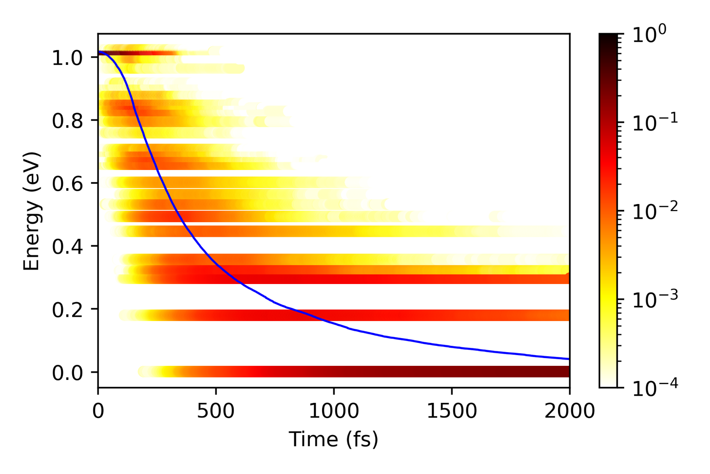
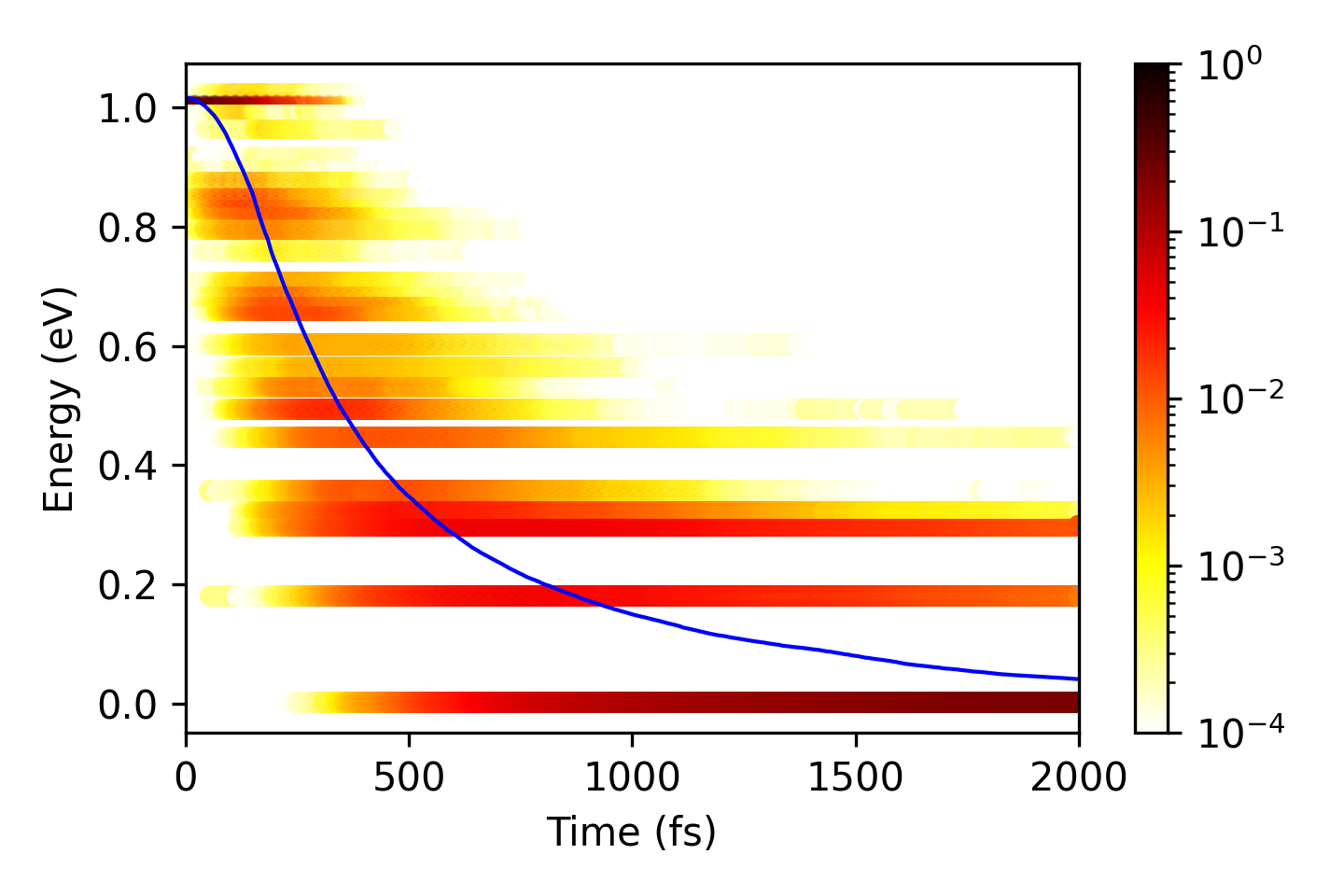
The electron plot uses the active-state populations in the three SHPROP.* files, averaged with equal weight. With \(a=(n,\mathbf k)\), the blue curve is the mean reference band energy:
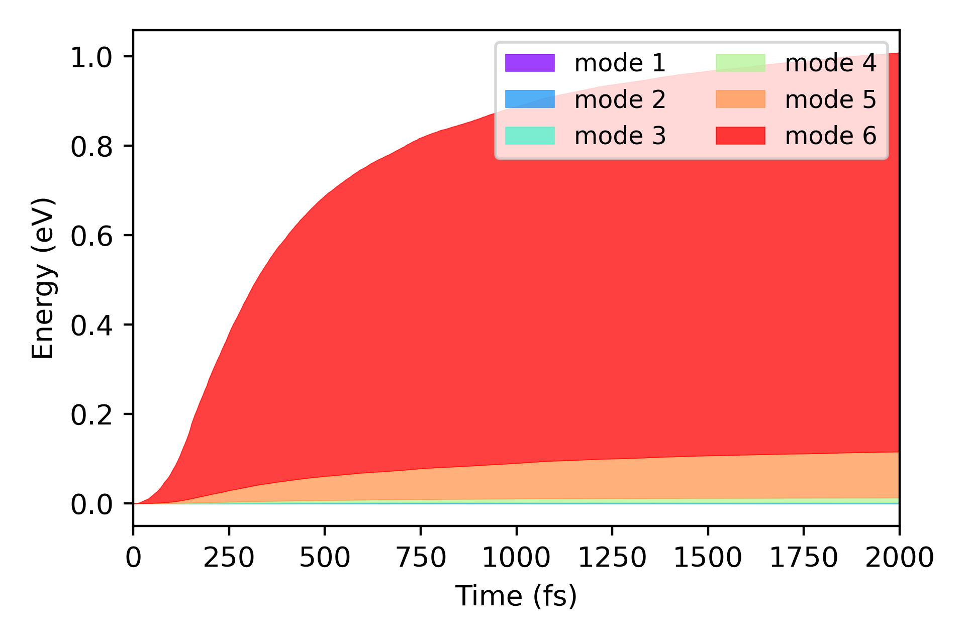
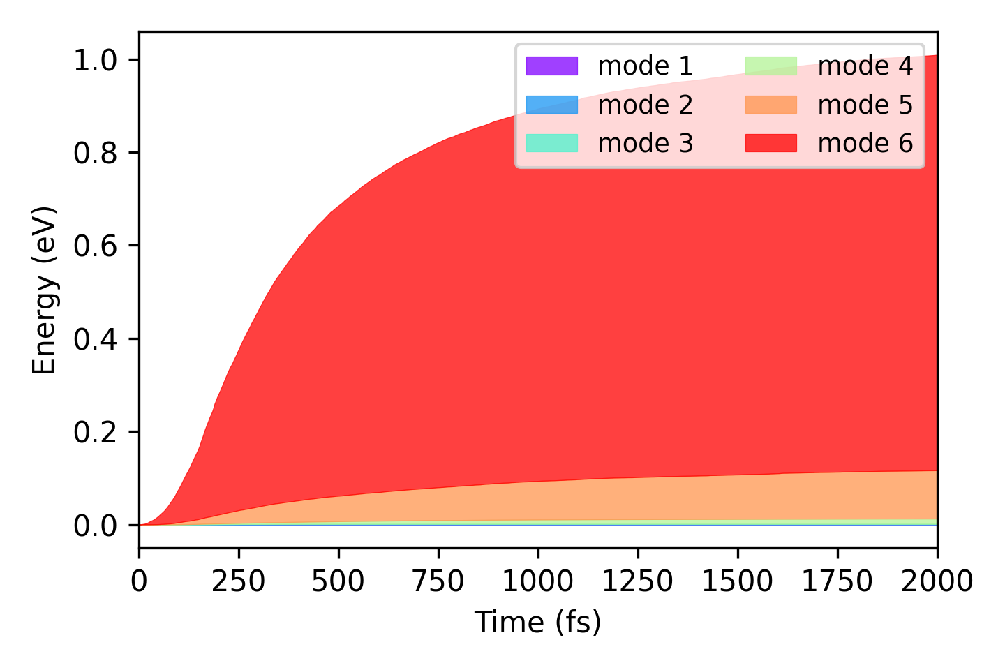
The plotting reference comes from the author's graphene band-plotting script. This observable is not the instantaneous eigenvalue of \(H_e(t)\), nor the full electron–nuclear energy. The PHPROP.* energy columns contain signed increments over successive 2 fs intervals. Sum them along time to obtain the cumulative net energy assigned to each phonon branch. These files already include the program's average over the three starting samples; dividing by three again would be incorrect.
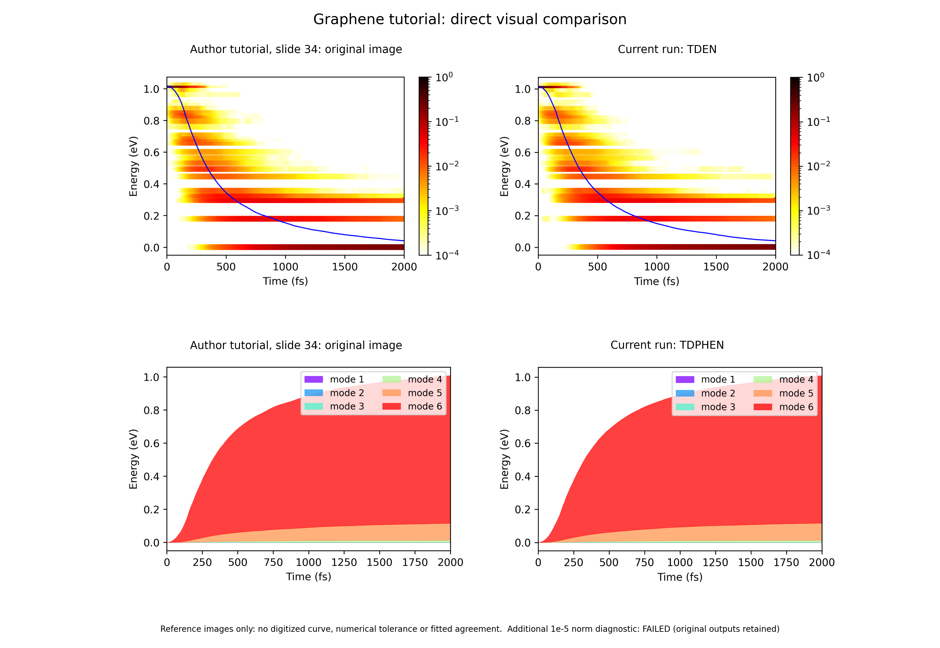
plot_tdprop and plot_tdphen functions. In the top row, the horizontal axis is time in fs; the vertical axis is reference band energy relative to −4.5302 eV; the logarithmic color scale gives active-state population, and blue gives its mean band energy. In the bottom row, the thickness of each colored region gives the cumulative net energy in that branch, in eV; the total is the top boundary. Red is branch 6 and orange is branch 5. The cooling trend and dominant branch agree visually. No reference curve was digitized or fitted. Open the image for full resolution.The run's mean active-state band energy falls from 1.01648 to 0.04048 eV relative to the plotting reference. At 2 ps, the cumulative net phonon energy is 1.00892 eV, including 0.89251 eV in branch 6 and 0.10376 eV in branch 5. This example therefore shows both electronic relaxation across the retained Bloch states and a strongly unequal distribution among phonon branches.
The original electron figure, original phonon figure, run electron figure, and run phonon figure are also available separately. The author figures retain their embedded image bytes. The run curves retain all 2001 electronic times at 1 fs spacing and all 1001 phonon times at 2 fs spacing, without interpolation or resampling: download the electronic CSV and phonon CSV.
8.5 Keep the estimator and validation limits visible
PSICT.* contains populations from the continuously propagated amplitudes, whereas SHPROP.* counts active hopping states. They are distinct estimators in this implementation. At 2 ps their mean reference band energies are approximately 0.70861 and 0.04048 eV, respectively. Substituting PSICT for SHPROP would change the result being compared with the tutorial.
Show the two electronic estimators and the phonon-energy curves
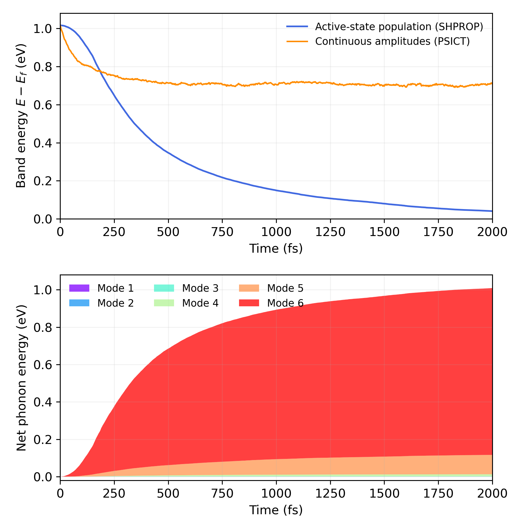
The maximum continuous-amplitude norm deviation was \(2.5818\times10^{-5}\), above an additional \(10^{-5}\) diagnostic chosen for this run; this threshold is not an author-specified tolerance. Original outputs and NELM were retained without renormalization. Also, the active-state band-energy loss is 0.97599 eV, about 0.03292 eV less than the cumulative phonon energy. With broadened channel assignments and prescribed phonon motion, these plots do not establish strict total-energy conservation or nuclear feedback.
The full-grid, original-parameter run and the visual comparison are complete. The tutorial does not supply reference curve arrays, a fixed random seed, or a numerical agreement tolerance, so pointwise numerical reproduction is not certified. Mesh, timestep, and sampling convergence were not established by this comparison. These limits are separate from successfully executing the example.
For the underlying analysis, see the author's output reader and plotting functions. The archived postprocessor used for the comparison requires the full NAMD outputs and the specified author sources; its input layout and scope are documented separately. The compact CSV consistency check runs on the published files alone:
python assets/code/hefeinamd_graphene_check.pyIt recomputes the quoted endpoint energies and checks time grids, the plotting offset, and the accumulated phonon increments. It performs no new dynamics and supplies no missing reference-data or convergence test.
9. Put the ingredients into a calculation
A practical EPC workflow follows the dependencies of the Hamiltonian:
- Choose the reference structure and electronic window. Compute the electronic states and establish the initial carrier state and observable.
- Compute lattice modes and electronic response. Density-functional perturbation theory (DFPT) provides harmonic modes and self-consistent perturbations. Wannier interpolation can then supply bands, phonons, and complex EPC matrix elements on finer compatible k/q grids.
- Define the nuclear preparation and path. Supply mode amplitudes and phases or a verified projection of an atomic trajectory. State the temperature, normalization, and feedback approximation.
- Construct and propagate \(H(t)\). Check momentum mapping, Hermiticity, band-window and grid convergence, the nuclear sampling interval, and the electronic integration step.
- Specify the statistical readout. Distinguish coherent populations from active-state occupations, state the switching and decoherence rules, and identify whether phonon quantities are prescribed coordinates or accumulated event statistics.
The documented upstream chain for HefeiNAMD-EPC uses Quantum ESPRESSO, Wannier90, qe2pert.x, and a compatible patched Perturbo to prepare *_ephmat_p*.h5 files for namd-epc. Perturbo's official interface guide describes the intermediate *_epr.h5 database; that database is not interchangeable with the EPC program's final matrix-element files. Wannier functions serve interpolation here; the carrier coefficients above are labelled by reference Bloch band and momentum.
The method is attractive when a periodic reference crystal and momentum-resolved scattering are central to the question. Large structural rearrangements, changing bonding, strong displacement dependence, or important nuclear feedback demand further modeling. In particular, replacing harmonic frequencies by a finite-temperature phonon spectrum does not by itself update the electronic derivatives or define the real-time nuclear ensemble.
The essential distinction from Part II is where the time-dependent electronic information comes from. The real-space route repeatedly evaluates instantaneous electronic states along nuclear configurations. The linear EPC route evaluates their reference response once, resolves it into modes, and multiplies that response by coordinates along a chosen path. Both routes still need the path, a converged state space, and a specified dynamical approximation.
10. FAQ: choosing and extending the EPC method
These questions compare the prescribed-path real-space workflow in Part II with the public EPC implementation inspected here. Method statements and source-code statements have different scopes: the latter refer to NAMDinMomentumSpace@689c952 and the real-space Hefei-NAMD@b7c8fc5, rather than every member of the software family.
- Which method should I choose for a particular process?
- How do the electronic Hamiltonians differ?
- How do their FSSH hopping rules differ?
- Which phonons are used, and can finite-temperature phonons replace them?
Q1. Which method should I choose for a particular process?
Start with the observable and the physical mechanism. EPC is a natural starting point when a periodic reference crystal, electronic momentum, and phonon-resolved scattering are central. Instantaneous-state real-space NAMD is often more convenient when local electronic character and structural fluctuations are central. This is a judgment about model suitability, not a universal accuracy ranking.
| Process and desired information | Useful starting point | What must still be checked |
|---|---|---|
| Hot-carrier cooling, intravalley or intervalley transfer, and the contributions of particular q points or phonon branches in a crystal | EPC, with explicit band/k labels and compatible k/q sampling | Whether a fixed reference and linear electronic response cover the sampled displacements; convergence of the state window, grids, and scattering broadening |
| Defect capture, interfacial transfer, or changes in the localization and layer character of electronic states | Real-space snapshots and NAC, with appropriate spatial or layer projections | Supercell size, thermal sampling, state tracking, and the approximations used for trapping or recombination; a changing band label alone is not charge transfer |
| Carrier dynamics strongly affected by anharmonic thermal distortions | Real-space NAMD on a suitable MD path, or an EPC extension driven by a verified anharmonic path | Classical MD is not quantum nuclear dynamics; an anharmonic path does not repair a first-order electronic expansion |
| Self-trapping, polaron formation, photoinduced structural changes, or reactions driven by the excited carrier | A model with suitable excited-state forces and electronic–nuclear feedback | Neither default prescribed-path route guarantees the carrier-induced lattice response. Large distortions may also invalidate the reference EPC expansion |
| Exciton dynamics, electron–hole recombination, or spin-selective processes | A branch with the required interacting or spin-dependent Hamiltonian | Neither the words “real space” nor “EPC” establish electron–hole interactions, spin–orbit coupling, or the required transition mechanism |
The authors' graphene study is an example of the first row: momentum and phonon-branch resolution explain the cooling mechanism. The official MoS₂/WS₂ tutorial results in Part II illustrate the instantaneous-state workflow. They do not establish that one method is always better for all crystals or interfaces.
A periodic defect or interface supercell can also serve as an EPC reference. The difficulty is practical and physical: the small-cell advantage may shrink, many bands may be required, and large structural changes can defeat a local displacement expansion. Conversely, real-space calculations can resolve primitive momenta through projection or unfolding if the supercell contains the relevant components. For a fair comparison, match the initial state, nuclear ensemble, electronic model, observable, and feedback assumptions before comparing relaxation times.
Q2. How do the electronic Hamiltonians differ?
Real-space NAMD uses a moving electronic basis; EPC uses a fixed reference basis and an approximate displaced electronic operator. “Adiabatic versus diabatic-like” describes the representation, but it does not describe all the approximations.
The key is whether the basis itself changes with time. In a fixed diabatic basis, only the expansion coefficients change, so the physical Hamiltonian matrix directly propagates them. In a moving adiabatic basis, both the coefficients and the basis states change. To see where the extra term comes from, expand the electronic state in an orthonormal basis:
Insert this derivative into \(i\hbar\,d|\Psi\rangle/dt=\hat H_e(t)|\Psi\rangle\) and project onto \(\langle\phi_a(t)|\). Moving the basis-derivative term to the right gives
Thus the coefficient propagation matrix is \(G=H-i\hbar d\): it accounts for both the physical Hamiltonian and the changing basis. The second term is required by the product rule; it does not add a new physical interaction. A fixed vector can likewise have changing components when the coordinate axes rotate.
For instantaneous adiabatic KS states, \(\hat H_e(t)|\phi_\beta(t)\rangle=\epsilon_\beta(t)|\phi_\beta(t)\rangle\), so the physical Hamiltonian matrix is diagonal:
The matrix that propagates the coefficients nevertheless contains the basis-motion contribution:
The off-diagonal NAC term transfers amplitude between instantaneous adiabatic states. It has units of inverse time; multiplication by \(-i\hbar\) gives an energy. Energies and wavefunction changes come from the sampled geometries, so this construction does not impose a first-order expansion in nuclear displacement. It still inherits electronic-structure, trajectory, finite-size, and retained-state errors.
In EPC's fixed reference Bloch basis, \(\partial_t|a;0\rangle=0\), so there is no basis-motion term: \(G^{\rm fixed}=H^{\rm fixed}\). The coupling caused by nuclear motion instead appears in the time-dependent off-diagonal Hamiltonian elements. This is the precise sense in which a fixed diabatic-like basis needs only the electronic Hamiltonian to propagate the coefficients; the decisive condition is that the basis is fixed, rather than its label alone. Here \(a,b\) label band-and-k pairs. With \(I\) collecting atomic displacement coordinates, the linear EPC approximation gives
The mode-resolved \(gQ/\ell\) formula in Section 5 is this linear displacement term written in phonon coordinates. Its off-diagonal elements are physical potential matrix elements in the fixed basis. The matrix elements \(g\) have energy units; they cannot be inserted in place of \(d\). The missing higher-order electronic terms remain missing even if the nuclear path is fully anharmonic.
If the two complete bases represent the same electronic operator along the same path, their generators are related by
This is a representation identity. A truncated linear EPC model and a snapshot calculation with a different path need not satisfy it as numerical models. The harmonic approximation for the nuclear potential and the classical-path approximation for feedback are separate choices. See Section 2 and the authors' coefficient equations.
Q3. How do their FSSH hopping rules differ?
The general population-current idea can be used in either representation. The inspected EPC code adds a static scattering-weight construction that is not identical to the current of its propagated Hamiltonian. Fixed Bloch states do not make a current-based switching rule impossible; directly substituting an energy-valued EPC matrix element into an adiabatic NAC formula would be incorrect.
For any orthonormal representation with coefficient equation \(i\hbar\dot z=Gz\) and Hermitian generator \(G\), define outward pair current by
The elementary fewest-switches construction uses the positive outward current, the source population, and a sufficiently short step. Appendix A derives each step, including the sign convention and the distinction between propagation and hopping states:
In the adiabatic basis this gives \(J_{a\to b}=2\,{\rm Re}[c_a^*d_{ab}c_b]\). In the fixed EPC basis it uses the instantaneous complex \(H^{\rm EPC}_{ab}(t)\). The inspected real-space routine uses the NAC-based expression, followed by a thermal correction. These are populations in the chosen basis; equivalent coefficient propagation does not make approximate stochastic switches invariant under arbitrary basis changes.
By contrast, EPC's calcEPC precomputes a nonnegative real quantity. For the inspected EPCTYPE=1 branch, its mode sum can be written as
Here \(g^0\) is the matrix element before the program's \(1/\sqrt{N_p}\) scaling, \(\mathbf q\) is the mapped momentum for the state pair, and \(\sigma\) is an energy broadening. This equation is a rewriting of the source expression, not a derivation of a new hopping theory. \(W\) has energy units. It is not already a transition rate, is not \(\sqrt W\), and is not \(H_{ab}(t)\). Squaring \(g\) removes its complex phase; the matching Gaussians select reference energy differences near a phonon energy. Both frequency channels carry \(n+1/2\) here, rather than the separate \(n\) and \(n+1\) weights of a textbook quantum absorption/emission rate.
The EPC switching routine then uses
Here \(\Delta t\) is the POTIM hopping interval, not an electronic substep. The coefficients still come from propagation with \(H^{\rm EPC}(t)\), so the switching statistics remain trajectory-dependent. However, \(W\) itself contains neither the instantaneous displacement nor its phase. It resembles a broadened second-order scattering weight, while the actual hopping expression also depends on electronic coherence. It should not be relabelled as a population-only golden-rule master equation or presented as the exact current of \(H^{\rm EPC}(t)\).
For an electron, the code sets \(B_{ab}=\exp[-(\epsilon_b^0-\epsilon_a^0)/(k_BT)]\) for upward transitions and one otherwise; the hole branch reverses the energetic direction. The real-space source also applies a Boltzmann suppression to uphill carrier transitions. These corrections do not establish exact quantum detailed balance or explicit energy exchange with moving nuclei. In the prescribed-path routes, a switch does not rescale the saved nuclear velocities. Full FSSH with nuclear feedback is a further model, explained in Part II.
Thus changing the phonon path while leaving \(W\) untouched creates a consistency question: propagation and switching would use different descriptions of the driving fluctuations. The fixed-basis formulation does not require this mismatch. A new trajectory-driven implementation must specify and validate its hopping rule as well as its Hamiltonian; changing only a phonon input is insufficient.
Q4. Which phonons are used, and can finite-temperature phonons replace them?
The documented default uses reference harmonic DFPT phonons with temperature-dependent occupation factors. A finite-temperature effective-phonon model can replace the harmonic lattice model, but a frequency list alone is not a complete replacement.
There are three different objects to keep separate:
- Reference harmonic modes. The standard QE →
qe2pertworkflow obtains a dynamical matrix and electronic perturbation potentials by density-functional perturbation theory at a specified reference structure. This is commonly called a zero-temperature harmonic calculation. More precisely, it is a reference-structure curvature calculation with the chosen electronic occupations and smearing; it is not an exact zero-temperature quantum-renormalized phonon spectrum. - Thermal occupations. In the inspected
EPCTYPE=1driver,TEMPenters the Bose factor and the amplitude \(\sqrt{n+1/2}\), while input frequencies remain fixed. Temperature also enters hopping acceptance, and sets the broadening whenSIGMA=0. None of these operations computes anharmonic frequency shifts. - Finite-temperature lattice dynamics. An effective dynamical matrix, quasiparticle frequencies, spectral peak weights, and linewidths are related but distinct. A set of effective frequencies and eigenvectors does not uniquely specify a full dynamical spectral function.
One practical route is an effective harmonic model at the target temperature. The temperature-dependent effective potential method (TDEP) and the stochastic self-consistent harmonic approximation (SSCHA) provide ways to obtain temperature-dependent lattice information. Perturbo already documents upstream interfaces: TDEP second-order force constants can enter qe2pert; SSCHA dynamical matrices can be supplied on the matching q grid. This is an existing interface in the current upstream documentation. It does not certify compatibility with the older patched Perturbo required by the inspected EPC program.
A consistent replacement must update the modes, their normalization, and the mode-resolved electronic couplings together. In the mass-weighted convention used above,
\(D^{\kappa j}_{ab}(\mathbf q)\) is the electronic response to a Cartesian displacement pattern; \(j\) is a Cartesian direction. To fix the Fourier normalization, use full-crystal-normalized reference states and define
This Fourier sum has no additional \(1/\sqrt{N_p}\) factor; that factor remains in the Hamiltonian of Section 5. The mode relation follows the usual EPC normalization. If the reference structure and Cartesian electronic derivatives are retained, those derivatives can be reprojected onto the new eigenvectors and rescaled: a new frequency does not by itself require recomputing every electronic derivative. This retains a reference electronic response; it does not calculate every finite-temperature correction to the electron–phonon interaction. If the structure, screening, or electronic model changes, their reuse needs separate justification. Keeping old \(g\) while arbitrarily changing \(\omega\), \(\ell\), and eigenvectors generally changes the electronic perturbation inconsistently.
The updated information must reach the interpolated EPC files, the coordinate driver, and the static hopping weights in Q3, with consistent q mapping and opposite-q phases. The author's Perturbo patch uses the mode eigenvectors and \(1/\sqrt{\omega}\) normalization when exporting \(g\); editing only a frequency dataset would leave these quantities inconsistent. This route includes an effective frequency renormalization. Independent undamped oscillators with those frequencies still do not generate phonon lifetimes, mode-to-mode energy redistribution, non-Gaussian fluctuations, or carrier-induced feedback. In SSCHA, the optimized auxiliary frequencies, the free-energy Hessian, and physical excitations from a dynamical response are distinct, as explained in the official spectral-function tutorial.
A second route is to keep an explicit anharmonic nuclear path. Given consistent Cartesian electronic derivatives, one can construct \(H(t)\) directly from the displacements, or project those displacements onto a complete mode basis. Finite-temperature modes can then serve as analysis coordinates; fitting a spectrum is not a mandatory step before constructing \(H(t)\). A complete change of coordinates with the derivatives transformed consistently leaves the linear electronic perturbation unchanged. Actual path amplitudes should not receive an additional \(\sqrt{n+1/2}\) multiplier.
For path-integral molecular dynamics (PIMD), the sampling clock is not physical real time: Fourier transforming an ordinary thermostatted PIMD trajectory does not give a physical phonon spectrum. Static quantum-correlation estimators can extract effective vibrational information, but require a specified estimator and do not supply real-time linewidths. Ring-polymer molecular dynamics (RPMD) instead supplies an approximate real-time route. Its bead internal modes are auxiliary degrees of freedom, so a bead-resolved Fourier spectrum cannot automatically be read as a set of physical phonons; spurious resonances in RPMD vibrational spectra are a known issue.
Using RPMD to drive the electrons would additionally require choosing a centroid, bead-resolved, or other electronic interface, defining the initial ensemble and hopping rule, and checking the target electronic observable. The repository's EPCTYPE=2 decomposition entry does not establish a verified end-to-end implementation of this extension. Effective finite-temperature phonons and explicit RPMD driving are therefore two different modeling routes, not interchangeable input switches.
The supported conclusion is that finite-temperature lattice information can enter upstream of the EPC Hamiltonian. It improves a specified part of the lattice model; it does not by itself remove linear-EPC truncation, define quantum electronic relaxation, or validate the current switching approximation.
Appendix A. Deriving hopping probabilities in diabatic and adiabatic bases
Why does a fixed-basis hopping formula contain the imaginary part of a Hamiltonian matrix element, while an adiabatic formula contains the real part of a nonadiabatic coupling? Both follow from the electronic population current. We first derive that exact current along a prescribed nuclear path, then introduce the stochastic fewest-switches prescription. The distinction matters: the Schrödinger equation fixes the population derivative, but does not by itself specify classical trajectories, active surfaces, or thermal acceptance factors.
A.1. Population current in a fixed orthonormal basis
Let \(\{|\chi_a\rangle\}\) be a time-independent orthonormal electronic basis. Along a nuclear path \(\mathbf R(t)\), define the Hermitian matrix \(H^{\rm D}\) of the represented electronic operator and its coefficients \(C_a\):
The superscript D denotes this fixed diabatic representation; it does not assume that the matrix is diagonal. Write its population as \(P_a^{\rm D}=|C_a|^2\). Differentiating both coefficient factors, substituting the Schrödinger equation, and using Hermiticity gives
The diagonal contribution vanishes because \(H^{\rm D}_{aa}\) is real. To make a positive sign mean population leaving state \(a\), define the outward pair current
This current has units of inverse time. Its antisymmetry conserves total electronic population. The minus sign belongs to the chosen outward convention; changing that convention without changing the probability formula would reverse the allowed hops.
A.2. From population current to a conditional hop probability
An active-state trajectory needs a nonnegative switching probability, whereas the quantum pair current can have either sign. The elementary fewest-switches choice permits switches only in the direction of the instantaneous net pair current. Let \(\lambda_{a\to b}\) be the conditional switching rate for a trajectory whose active state is \(a\), and let \([x]_+=\max(x,0)\). Matching its outgoing ensemble flow to the positive quantum current gives
Here \(\Delta t\) is a sufficiently short switching interval and \(P_a^{\rm D}>0\). The denominator converts an ensemble population flow into a probability conditioned on already occupying the active state. The total outgoing probability must not exceed one; smaller steps or integrated rates are needed if it does. The probability to stay is one minus that total.
The matching can be checked directly. Consider replicas with the same prescribed nuclear path and electronic wavefunction, and let \(f_a\) be their active-state fraction. Their continuous-time balance equation is
Thus matched initial fractions reproduce the electronic populations in this shared-path, continuous-time construction. Finite switching steps introduce discretization error. When different active surfaces generate different nuclear paths, this simple shared-wavefunction argument no longer establishes exact ensemble populations. The stochastic prescription is an additional modeling step beyond the exact population-current identity.
The probability depends on electronic coherence and its phase relative to the coupling. It is not proportional to \(|H_{ab}|^2\) alone. A golden-rule rate arises only after additional perturbative and statistical assumptions; it is a different reduction of the dynamics.
A.3. Why the adiabatic formula uses a real part
In the instantaneous adiabatic basis, write the same electronic state with coefficients \(c_a\). The physical Hamiltonian is diagonal, while the basis motion contributes to the coefficient generator, as derived in Q2:
To distinguish the time and spatial derivatives, denote the time coupling by \(\tau_{ab}\) here. It is the quantity called \(d_{ab}(t)\) in Q2. The spatial derivative coupling is the vector \(\mathbf d^{R}_{ab}\):
Orthonormality implies \(\tau^\dagger=-\tau\), so \(G^{\rm A}\) is Hermitian. Applying the same population-current identity to \(P_a^{\rm A}=|c_a|^2\), the off-diagonal generator gives
The real part appears because the generator contains \(-i\hbar\tau_{ab}\). The fixed-basis expression uses an energy-valued \(H^{\rm D}_{ab}\); the adiabatic expression uses an inverse-time \(\tau_{ab}\). They implement the same outward-current construction in different population bases. An energy-valued EPC matrix element cannot replace \(\tau_{ab}\) in the second formula.
A.4. The propagation basis does not fix the hopping states
A program can propagate coefficients in a fixed basis while assigning active states to instantaneous adiabatic surfaces. To do that consistently, it must transform the coefficients and obtain the couplings for the states between which it actually switches. For a unitary matrix \(U\) whose columns are the adiabatic eigenvectors in the same fixed electronic space,
Adiabatic hopping therefore uses the transformed \(c_\alpha\) and adiabatic time couplings. Hopping among fixed states uses the \(C_a\) and fixed-basis current instead. The two coefficient equations can describe identical electronic evolution, while the two sets of populations describe different projectors. Approximate surface-hopping dynamics also depends on the active-state forces and nuclear momentum adjustment, so it is not generally invariant under changing the hopping basis. The current formula alone does not determine those nuclear rules.
A.5. An exact two-state check of the distinction
Hold the nuclei fixed and take a real constant \(V>0\). This analytically solvable example checks the current's sign and shows why fixed-state transfer need not mean a jump between energy eigenstates:
The fixed-state populations oscillate, and the derived outward current has exactly the required sign:
During the first interval in which \(P_1^{\rm D}\) decreases, this current permits switches from 1 to 2. When the current reverses, the permitted direction reverses. At zero source population the conditional expression is undefined; the shared-path construction assigns no trajectories to that empty state.
The energy eigenstates and their populations tell a different, equally consistent story:
No adiabatic population current or adiabatic hop is required. The oscillation in the fixed basis comes from the evolving relative phase of the two energy eigenstates. The two descriptions agree on the electronic state; they count populations of different states. This is an analytic check, not a material simulation or a new reproduction of the graphene tutorial.
A.6. What this derivation does and does not imply for EPC
For a fixed reference Bloch basis, the current consistent with propagation by \(H^{\rm EPC}(t)\) follows A.1–A.2 with its instantaneous complex matrix elements. The fixed basis creates no mathematical need to replace those elements by static scattering weights.
The inspected calcprop_EPC_mpi routine instead uses the precomputed \(W_{ab}\) and a thermal factor described in Q3. That is an additional implementation choice, not the fixed-basis current derived here. Neither \(W_{ab}\) nor a Boltzmann penalty follows merely by changing from an adiabatic to a diabatic representation. Adding an acceptance factor changes the matched population flows, so it requires its own physical justification and validation.
The algebra above establishes the electronic current and its elementary fewest-switches interpretation. It does not establish exact coupled electron–nuclear dynamics, quantum detailed balance, or the validity of a particular EPC switching model. The method's original reference is Tully's 1990 fewest-switches paper; the derivation here makes the outward-current convention and the representation choice explicit.
Sources and further reading
- Z. Zheng et al., Ab initio real-time quantum dynamics of charge carriers in momentum space, Nature Computational Science 3, 532–541 (2023); author manuscript, especially Eqs. (5)–(11).
- J. C. Tully, Molecular dynamics with electronic transitions, Journal of Chemical Physics 93, 1061–1071 (1990): the original fewest-switches surface-hopping method.
- EPW theory documentation: Bloch normalization, phonon coordinates, self-consistent perturbations, and EPC conventions. The mass-weighted coordinate convention is stated explicitly in this article.
- HefeiNAMD-EPC source snapshot, commit
689c952: implementation statements above refer to this version, rather than every program called momentum-space NAMD. - Quantum ESPRESSO to Perturbo and interpolation of bands, phonons, and EPC matrix elements.
- Perturbo interfaces to TDEP and SSCHA; SSCHA spectral-function tutorial: effective lattice matrices and physical spectra have distinct roles.
- T. Morresi et al., Probing anharmonic phonons by quantum correlators: A path integral approach; M. Rossi, M. Ceriotti, and D. E. Manolopoulos, How to remove the spurious resonances from ring polymer molecular dynamics.
- NAC and moving-basis foundations; Part II's real-space construction and FSSH.