CMD Effective Surfaces for Tully SAC

This note builds a centroid molecular dynamics (CMD) effective surface for Tully's simple avoided crossing, then uses that surface in Ehrenfest and fewest-switches surface hopping dynamics. The central object is not a new nonadiabatic coupling formula, but a state-resolved potential of mean force obtained from constrained path-integral Monte Carlo.

Why a CMD Surface?

A classical mixed quantum-classical trajectory samples one nuclear point \(Q\) at a time. Near a narrow avoided crossing, however, a quantum nuclear packet can delocalize across the coupling region. CMD folds part of this nuclear quantum delocalization into an effective free-energy surface for the centroid coordinate. In a one-dimensional two-state benchmark this is a useful diagnostic: far from the avoided crossing the CMD surface should reduce to the ordinary adiabatic energy, while near the coupling region the lower-state barrier can be softened by imaginary-time delocalization.

The implementation used here is deliberately conservative. It precomputes the CMD potential of mean force (PMF) on an adaptive grid, aligns the PMF in the non-coupled reactant asymptote, interpolates a continuous energy-force pair, and only then runs Ehrenfest and FSSH trajectories. It is not an on-the-fly PIMC calculation during dynamics.

Constrained PIMC on One Adiabatic State

For each adiabatic state \(s\) and centroid value \(Q\), a ring-polymer path \(\{q_i\}_{i=1}^{P}\) is sampled under the exact centroid constraint

Q=\frac{1}{P}\sum_{i=1}^{P}q_i .

The state-resolved Euclidean action is

S_s(\mathbf q)= K_P(\mathbf q)+U_{P,s}(\mathbf q).

K_P(\mathbf q)= \frac{1}{2\beta_P} \sum_{i=1}^{P} m(q_{i+1}-q_i)^2

U_{P,s}(\mathbf q)= \beta_P\sum_{i=1}^{P} E_s(q_i), \qquad \beta_P=\frac{\beta}{P}.

The Metropolis move changes one bead, then shifts the entire path so that the centroid returns exactly to \(Q\). This keeps the constrained ensemble well defined without adding a penalty potential. In this benchmark the highest PMF level used \(P=8\) beads and \(15000\) Monte Carlo steps per grid point and state. The adaptive centroid grid has 66 points over \([-7,7]\), with spacing \(0.1\) in the coupling region \([-2.221,2.221]\) and spacing \(0.5\) outside.

Mean Force and PMF Integration

The PMF is reconstructed from a constrained mean force, not from a simple average of adiabatic energies. For a sampled path, the bead-averaged force on state \(s\) is

\bar F_s(\mathbf q)= \frac{1}{P}\sum_{i=1}^{P}F_s(q_i), \qquad F_s(q)=-\frac{\partial E_s(q)}{\partial q}.

The CMD force is the constrained ensemble average

F_s^{\mathrm{CMD}}(Q)= \left\langle \bar F_s(\mathbf q)\right\rangle_{Q,s}.

The state-resolved PMF \(A_s(Q)\) is then obtained by integrating

\frac{dA_s(Q)}{dQ}=-F_s^{\mathrm{CMD}}(Q).

A_s(Q_j)=A_s(Q_0) -\int_{Q_0}^{Q_j} F_s^{\mathrm{CMD}}(Q)\,dQ .

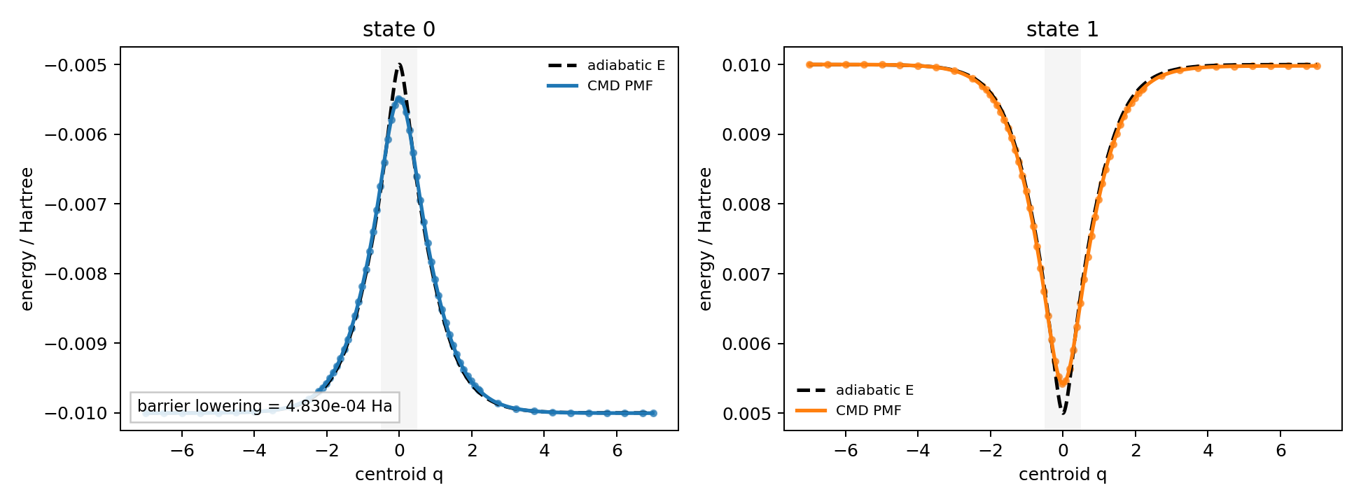
Because a PMF is defined only up to a constant, each state is aligned by a least-squares shift in the reactant asymptote \(Q\le -3\). This is important: aligning at \(Q=0\) would pin the avoided crossing itself and hide the barrier lowering that CMD is meant to reveal. After asymptotic alignment, the residual mismatch in the left non-coupled region is about \(3\times 10^{-6}\) hartree.

CMD PMF compared with ordinary adiabatic energies for Tully simple avoided crossing — CMD PMF surfaces compared with ordinary adiabatic energies. The horizontal axis is the centroid coordinate \(Q\); the vertical axis is energy in hartree. Dashed black curves are ordinary adiabatic energies and colored solid curves are CMD PMFs. The gray band marks \(|Q|\le 0.5\), the barrier region used for the numerical estimate. The lower state is nearly unchanged in the asymptotic region but is lowered around the avoided crossing by \(4.83\times 10^{-4}\) hartree, consistent with a quantum-delocalization reduction of the effective reaction barrier.

The classical counterpart—and the ensemble distinction

For a classical Cartesian coordinate \(x\) and remaining coordinates \(y\), define \(Z_x=\int dy\,e^{-\beta U(x,y)}\) and \(F(x)=-\beta^{-1}\ln Z_x+C\). Differentiating under the integral gives

\begin{aligned} F'(x)&=-\beta^{-1}\frac{Z_x'}{Z_x}\\ &=\frac{\int dy\,(\partial_xU)e^{-\beta U}} {\int dy\,e^{-\beta U}}\\ &=\langle\partial_xU\rangle_x. \end{aligned}

This explains the common mean-force logic, but not an identity of the two ensembles. The CMD average above constrains a quantum path's centroid; this classical average constrains a physical coordinate. Nonlinear collective variables also require their geometric measure. Reaction Computation IV uses the classical case to isolate entropy and test umbrella reconstruction.

Interpolating a Continuous \(E(Q)\) and \(F(Q)\)

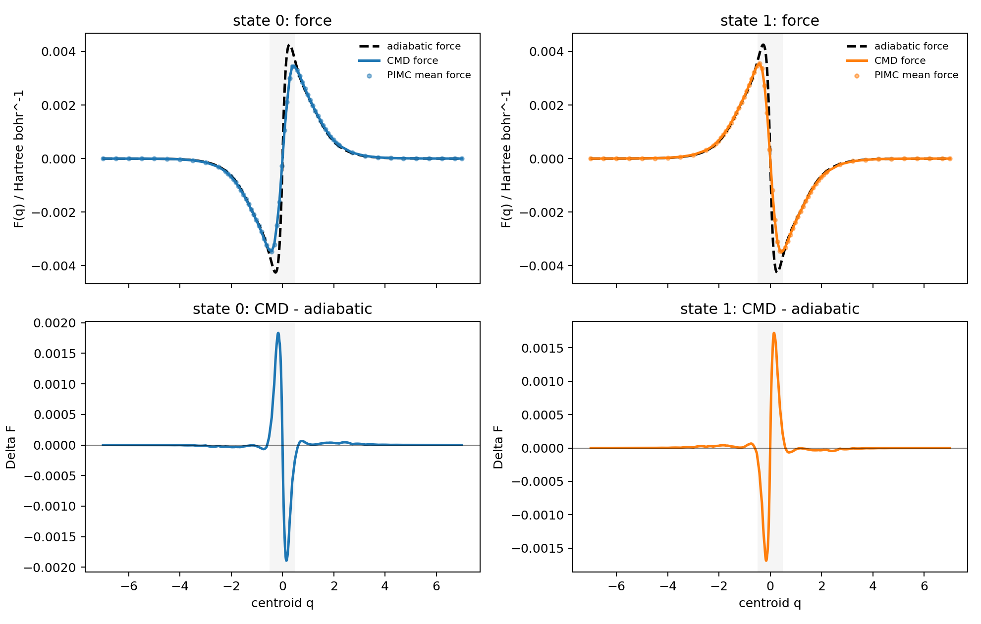
Dynamics cannot run directly on isolated PMF grid values. The surface must provide a continuous energy and a force that is consistent with that energy. The benchmark therefore uses a cubic Hermite spline for each state:

E_s^{\mathrm{CMD}}(Q) = H_s\!\left(Q;\, A_s(Q_i),\, A_s'(Q_i)\right).

A_s'(Q_i)=-F_s^{\mathrm{CMD}}(Q_i).

The force used in dynamics is the derivative of the same spline,

F_s^{\mathrm{dyn}}(Q) = -\frac{dE_s^{\mathrm{CMD}}(Q)}{dQ}.

This avoids a common inconsistency: fitting energy and force with two unrelated splines can produce a trajectory force that is not the derivative of the plotted surface. In the present implementation the diagonal energies and diagonal forces are replaced by the CMD effective values, while the adiabatic wavefunctions and derivative couplings are still evaluated from the original Tully model at the centroid.

CMD force compared with ordinary adiabatic force and their difference — Force-level comparison. Top panels show the ordinary adiabatic force (black dashed), the Hermite-interpolated CMD force (solid), and the PIMC mean-force grid points. Bottom panels show \(F_{\mathrm{CMD}}-F_{\mathrm{adiabatic}}\). The correction is localized near the avoided crossing; in the left asymptote \(Q\le -3\), the maximum force difference is only about \(1.3\times 10^{-5}\) hartree bohr\(^{-1}\), while in \(|Q|\le0.5\) it reaches about \(1.9\times10^{-3}\) on state 0.

Dynamics on the CMD Surface

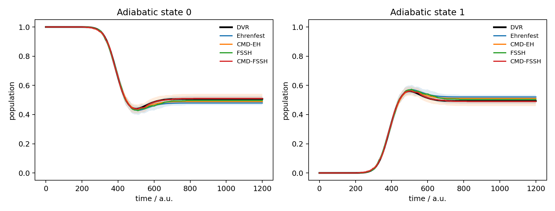
The same initial ensemble is used for ordinary and CMD dynamics: a boosted harmonic thermal density centered at \(q_0=-4\), mean momentum \(p_0=20\), mass \(M=2000\), temperature \(300\) K, and preparation frequency \(\omega=0.004\) a.u. The quantum reference is a DVR density-matrix propagation on Tully's simple avoided crossing. The trajectory methods propagate to \(t=1200\) a.u.; this is long enough for the packet to leave the coupling region and for the final DVR population to plateau.

For Ehrenfest, the nuclear force is the electronic-population-weighted average of the CMD state forces. For FSSH, each trajectory moves on an active CMD surface, while hop probabilities still use the original derivative coupling evaluated at the centroid. The calculation is therefore a minimal CMD effective-surface correction, not a complete path-integral nonadiabatic theory.

DVR, Ehrenfest, CMD-Ehrenfest, FSSH, and CMD-FSSH population comparison — Population comparison for \(t\in[0,1200]\) a.u. The black curve is the DVR total adiabatic population, blue is ordinary Ehrenfest, orange is CMD-Ehrenfest, green is ordinary FSSH, and red is CMD-FSSH. The FSSH bands show two standard errors for the 1024-trajectory run. CMD-Ehrenfest reduces the final-state and time-series error relative to ordinary Ehrenfest.

Benchmark Numbers

The PMF convergence check compares \(5000\) and \(15000\) PIMC steps per centroid point and state. The maximum PMF difference is \(8.89\times10^{-5}\) hartree and the RMS difference is \(4.41\times10^{-5}\) hartree. The lower-state barrier lowering measured from the left reactant basin is \(4.83\times10^{-4}\) hartree.

Method	Trajectories	Final \(P_1\)	DVR final \(P_1\)	Final absolute error	RMS error vs DVR
DVR	-	0.492785	0.492785	0	0
Ehrenfest	1024	0.520624	0.492785	0.027839	0.020349
CMD-Ehrenfest	1024	0.510500	0.492785	0.017715	0.012802
FSSH	4096	0.500488	0.492785	0.007703	0.007962
CMD-FSSH	4096	0.505859	0.492785	0.013074	0.010601

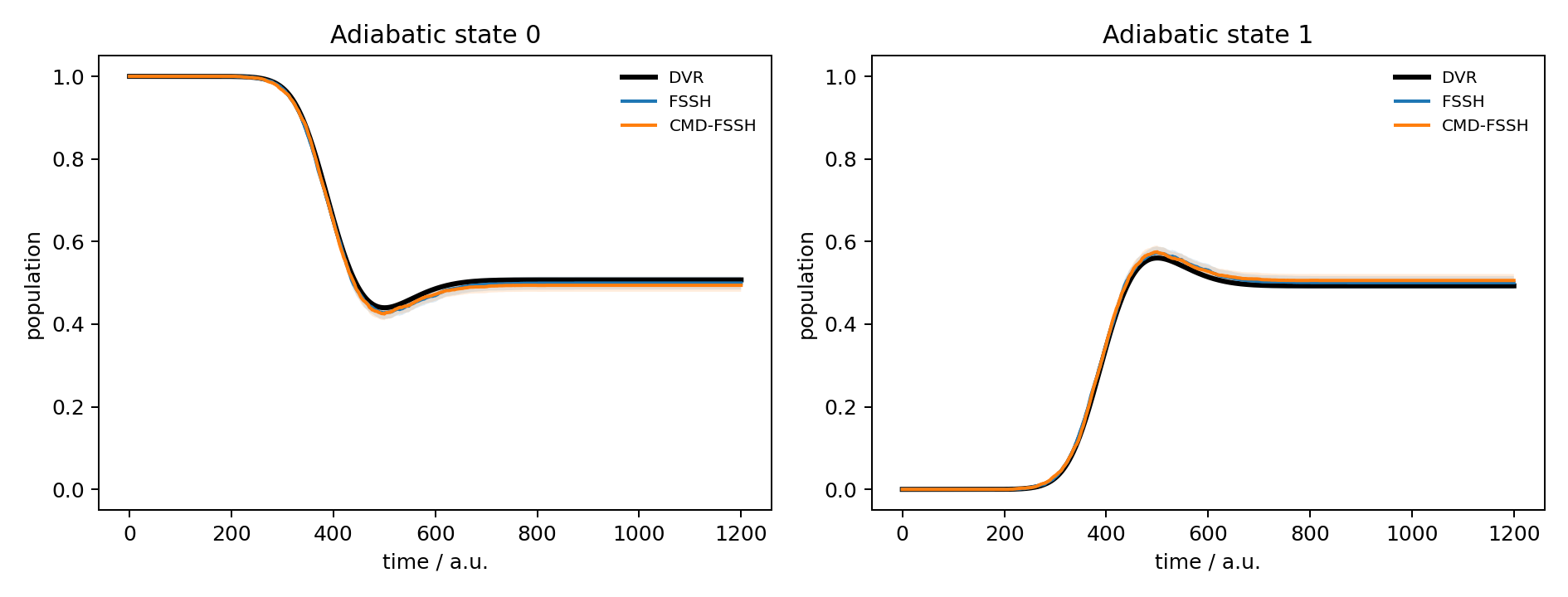
Two points are worth keeping separate. First, CMD-Ehrenfest improves the Ehrenfest result for this setup. Second, CMD-FSSH is not automatically superior to ordinary FSSH after trajectory convergence: the 4096-trajectory extension gives a smaller prefix RMS convergence error for CMD-FSSH, but the final RMS error against DVR is slightly larger than ordinary FSSH. The CMD surface is physically interpretable, but it is not a universal correction for every MQC closure.

FSSH and CMD-FSSH compared with DVR using 4096 trajectories — FSSH-only extension to 4096 trajectories. The black line is the DVR reference, blue is ordinary FSSH, and orange is CMD-FSSH. Both trajectory methods reach a stable asymptotic population; the 2048-to-4096 prefix RMS difference is \(7.74\times10^{-3}\) for FSSH and \(2.82\times10^{-3}\) for CMD-FSSH.

DVR Reference and Monotonicity

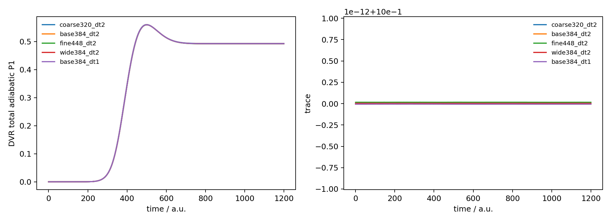
The DVR reference itself was checked against grid, box, and time-step changes. Relative to the \(N_{\mathrm{DVR}}=384\), \(x_{\max}=18\), \(\Delta t=2\) baseline, the final \(P_1\) changes by \(5.44\times10^{-4}\) for \(N_{\mathrm{DVR}}=320\), \(4.22\times10^{-4}\) for \(N_{\mathrm{DVR}}=448\), \(1.21\times10^{-4}\) for \(x_{\max}=22\), and zero to printed precision when halving the time step to \(\Delta t=1\). The density trace is conserved to about \(10^{-14}\).

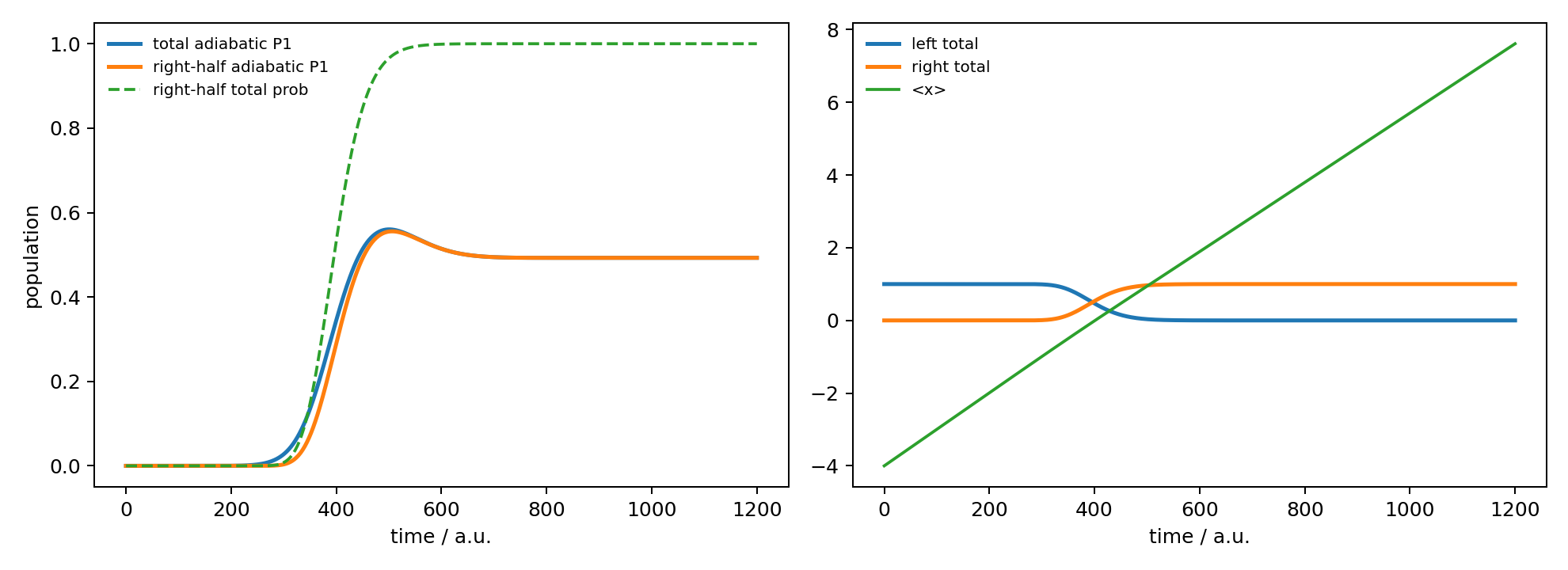
The plotted DVR quantity is the total instantaneous adiabatic population \(P_1(t)\), not a cumulative transmitted flux. It is therefore not required to be monotonic: it overshoots near \(t=500\) a.u. and relaxes to the asymptotic value. This overshoot is also converged. In contrast, the right-half total probability is monotonic and reaches \(0.99999996\), confirming that the packet has scattered out of the coupling region.

DVR convergence of total adiabatic P1 and trace — DVR convergence for the total instantaneous adiabatic \(P_1(t)\). The left panel overlays five grid, box, and time-step choices; the curves are visually indistinguishable on the population scale. The right panel shows trace conservation. The nonmonotonic peak is therefore a converged property of this observable, not a grid artifact.

DVR total adiabatic population compared with right-half probability — Total versus split DVR observables. The total adiabatic \(P_1(t)\) and the right-half adiabatic \(P_1(t)\) both show an avoided-crossing overshoot, whereas the right-half total probability is monotonic and approaches one. This separates a monotonic scattering-arrival diagnostic from an instantaneous adiabatic-population diagnostic.

Code and Data

cmd_sac_benchmark.py builds the adaptive CMD PMF, runs DVR, Ehrenfest, FSSH, CMD-Ehrenfest, and CMD-FSSH, and writes the main population figures.
cmd_sac_extend_fssh.py reuses a saved CMD PMF and DVR result to extend the FSSH and CMD-FSSH trajectory convergence to 4096 trajectories.
cmd_sac_dvr_convergence.py runs the DVR-only grid, box, and time-step convergence diagnostics.
cmd-sac-summary.csv stores the 1024-ensemble EH/CMD-EH/FSSH/CMD-FSSH comparison.
cmd-sac-fssh4096-summary.csv stores the 4096-trajectory FSSH and CMD-FSSH comparison.
cmd-sac-pimc-diffs.csv stores the PIMC PMF convergence difference.
cmd-sac-barrier-metrics.csv stores the PMF barrier-lowering metrics.
cmd-sac-dvr-convergence-metrics.csv and cmd-sac-dvr-convergence-vs-base.csv store the DVR convergence evidence.

CMD series map

Part I: CMD Effective Surfaces for Tully SAC - constrained PIMC PMFs used as state-resolved effective surfaces for one-dimensional nonadiabatic dynamics.
Part II: Curvature Red Shift in a 2D Morse Bottle - a curved multidimensional surface where the same centroid construction produces an artificial-instanton basin and a red-shifted CMD spectrum.
Part III: Learning Centroid Forces - mean-force derivation, direct/delta learning, and molecular dataset construction.