DVR VI: Flux-Side Kubo Correlation

The flux-side correlation function is a rate-like observable. It asks how much probability crosses a dividing surface and later remains on the product side. In DVR, that idea becomes a side projector, a commutator-defined flux operator, and a thermal Kubo weight.

Classical picture

The classical flux-side form is

C_{fs}(t)=\langle F(0)h(t)\rangle, \qquad h(t)=\Theta(x(t)-s), \qquad F(0)=\delta(x(0)-s)\dot x(0).

For free motion \(x(t)=x_0+vt\), the delta function selects trajectories starting at the dividing surface and the side function checks whether they are on the product side at time \(t\).

Quantum side and flux operators

The side operator is

\hat h=\Theta(\hat x-s)\otimes I_{\mathrm{el}}.

The flux operator follows from the Heisenberg time derivative of \(h(t)\):

\hat F=\frac{d\hat h(t)}{dt}\bigg|_{t=0} = \frac{i}{\hbar}[\hat H,\hat h].

In an energy basis, this also implies \(F_{nm}=\frac{i}{\hbar}(E_n-E_m)h_{nm}\) when the same Hamiltonian defines the basis.

Kubo flux-side formula

The Kubo-transformed flux-side expression used in the source notes is

C_{\mathrm{fs}}^{\mathrm{Kubo}}(t;\beta)= \frac{1}{\beta}\int_0^\beta d\lambda\, \mathrm{Tr}\!\left[ e^{(\lambda-\beta)H}F_1 e^{(-\lambda+it/\hbar)H}h_2 e^{-iHt/\hbar} \right].

Inserting energy eigenstates gives the same thermal kernel as the position Kubo note:

C_{\mathrm{fs}}^{\mathrm{Kubo}}(t;\beta)= \sum_{mn}W_{mn}F_{mn}h_{2,nm} e^{i(E_n-E_m)t/\hbar},

W_{mn}= \begin{cases} \dfrac{e^{-\beta E_n}-e^{-\beta E_m}}{\beta(E_m-E_n)},& m\ne n,\\ e^{-\beta E_m},& m=n. \end{cases}

Why compute flux-flux first?

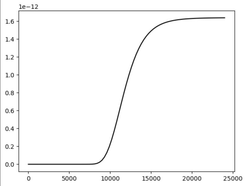
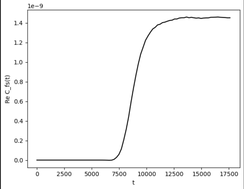
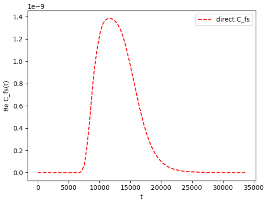
The direct \(C_{fs}\) calculation can decay when a complex absorbing potential removes amplitude after the packet reaches the absorbing region. A more stable route is to compute the flux-flux correlation and then integrate:

\frac{d}{dt}C_{fs}(t)=C_{ff}(t), \qquad C_{fs}(t)=\int_0^t C_{ff}(\tau)\,d\tau.

The source note uses the real Hamiltonian for the thermal Kubo weighting and the absorbing Hamiltonian only for real-time propagation. This keeps the Boltzmann kernel physical while damping boundary reflections during the real-time part.

CAP and Schur propagation

With a complex absorbing potential, the propagation Hamiltonian is non-Hermitian:

H_{\mathrm{abs}}=H-i\Gamma W(x).

The source workflow uses a complex Schur decomposition,

H_{\mathrm{abs}}=ZTZ^\dagger,

so real-time factors can be evaluated with the triangular matrix \(T\). This is numerically safer than relying directly on ill-conditioned eigenvectors of a non-normal matrix.

Numerical results

Flux-side correlation plateau for small coupling — Flux-side signal for one parameter set. The horizontal axis is time and the vertical axis is the real part of \(C_{fs}\). The black curve rises from near zero and approaches a plateau, which is the rate-like long-time value after successful crossings have been accumulated.

Flux-side Kubo correlation plateau for SAC model — DVR flux-side Kubo result for the simple avoided crossing setup. The black curve again reaches a stable plateau. Compared with the first panel, the scale is larger because the parameter set and thermal weighting differ.

Direct flux-side correlation curve — Direct \(C_{fs}\) diagnostic. The red dashed curve is localized in time instead of approaching a stable plateau. This illustrates the practical problem: after the wavepacket reaches the absorbing region, the side expectation can decay even though the crossing event has already occurred.

Operator implementation

def side_projector(x, dividing_surface=0.0):
    return np.diag((x > dividing_surface).astype(float))

def flux_operator(hamiltonian, side, hbar=1.0):
    return 1j / hbar * (hamiltonian @ side - side @ hamiltonian)

The flux-side calculation combines the pieces built earlier in the series: Part I establishes the finite Hamiltonian, Part II identifies the side and flux matrices, Parts III-IV describe pure-state and density-matrix propagation, and Part V supplies the thermal Kubo spectral kernel. Part VII reuses this machinery with local adiabatic projectors to form a population-resolved transfer diagnostic.

Code used in this note

dvr_kubo_minimal.py contains the shared side projector, flux commutator, and Kubo kernel.
source/flux-side-kubo/utils/quantum.py preserves the flux-side quantum utility routines from the working code folder.
source/flux-side-kubo/utils/classical.py contains the matching classical helper routines used for comparison tests.
source/flux-side-kubo/reference-data/Cfs_real_data.txt, Cfs_real_data_adi.txt, and Cfs_real_data_dia.txt are the small reference datasets used while checking the flux-side curves.

DVR series map

Part I: Wavepacket Dynamics Methods - discretization choices and the harmonic-oscillator benchmark.
Part II: Operator Matrices in the DVR Basis - matrix structure behind kinetic, side, and flux operators.
Part III: Wavepacket Dynamics with DVR - exact finite-dimensional propagation of a prepared wavepacket.
Part IV: Density-Matrix Ensemble Evolution - thermal ensembles, filtering, and absorber bookkeeping.
Part V: Kubo-Transformed Position Correlation - spectral thermal correlation functions.
Part VI: Flux-Side Kubo Correlation - rate-like observables from side and flux operators.
Part VII: Excited-Ground Kubo Population Correlation - local adiabatic projectors and population-resolved transfer diagnostics.