The useful thing about DVR is that the important quantum operators become inspectable matrices. Kinetic energy is dense and structured, local potentials are diagonal, side operators are projectors, and flux operators appear as commutators around a dividing surface.

Kinetic energy

Use equally spaced points \(x_i=x_{\min}+i\Delta x\). The cardinal basis \(\phi_i(x)=\Delta x^{-1/2}\operatorname{sinc}[\pi(x-x_i)/\Delta x]\), with \(\operatorname{sinc}u=\sin u/u\), gives diagonal coordinate and potential matrices under DVR quadrature. Its band-limited Fourier representation supplies the kinetic matrix:

\[ T_{ij}=\frac{\Delta x}{2\pi} \int_{-\pi/\Delta x}^{\pi/\Delta x} \frac{\hbar^2k^2}{2m}e^{ik(x_i-x_j)}\,dk. \]

Set \(u=k\Delta x\) and \(n=i-j\). The remaining integral is elementary:

\[ \frac1{2\pi}\int_{-\pi}^{\pi}u^2e^{inu}\,du =\begin{cases} \pi^2/3,&n=0,\\ 2(-1)^n/n^2,&n\ne0. \end{cases} \]

The off-diagonal result follows by two integrations by parts. Substitution gives the infinite-domain sinc convention used in the code:
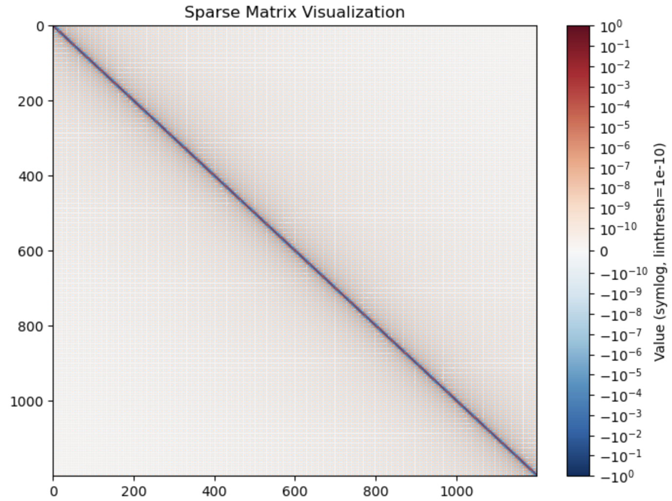
\[ T_{ii'}=\frac{\hbar^2}{2m\Delta x^2}(-1)^{i-i'} \begin{cases} \pi^2/3,& i=i',\\ 2/(i-i')^2,& i\ne i'. \end{cases} \]
Sinc DVR kinetic matrix heat map
Sinc DVR kinetic-energy matrix. Both axes are DVR grid indices. The color scale is logarithmic in the signed matrix value: the diagonal is dominant, and off-diagonal elements alternate sign while decaying away from the diagonal. This is the visual fingerprint of a nonlocal spectral kinetic operator.

Multi-state Hamiltonian blocks

For a diabatic model with electronic indices \(a,b\), the product-basis Hamiltonian is

\[ H_{(i,a),(j,b)}=\delta_{ab}T_{ij}+\delta_{ij}V_{ab}(x_i). \]

The first term repeats the same nuclear kinetic matrix on each electronic-state block. The second term is diagonal in the DVR grid but may couple different electronic states at the same grid point.
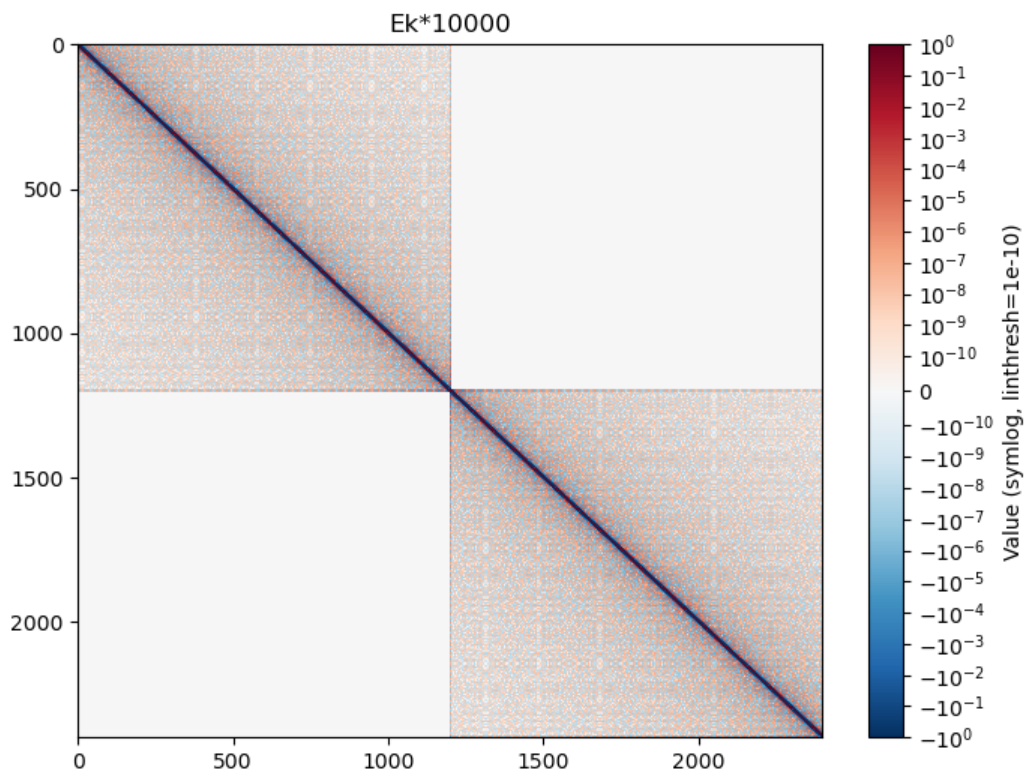
Kinetic blocks in a two-state DVR matrix
Two-state kinetic block structure. The upper-left and lower-right blocks are copies of the same nuclear kinetic matrix. The blank off-diagonal state blocks show that the kinetic operator does not itself change the electronic state.
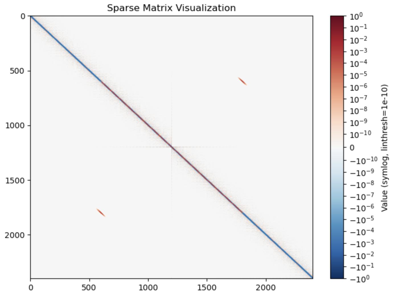
Full Hamiltonian heat map
Full Hamiltonian matrix. The two diagonal blocks contain \(T+V_{11}(x)\) and \(T+V_{22}(x)\). The smaller off-diagonal features come from the local diabatic coupling \(V_{12}(x)\), which appears only at equal grid indices.

Projectors and side operators

A side operator marks whether the nuclear coordinate lies to one side of a chosen dividing surface \(s\):
\[ h=\Theta(\hat x-s)\otimes I_{\mathrm{el}}. \]
Adiabatic ground-state projector matrix
Ground-state projector in a two-state calculation. The nonzero pattern follows the selected local adiabatic component rather than a simple coordinate step. It is useful for separating electronic-state-resolved population.
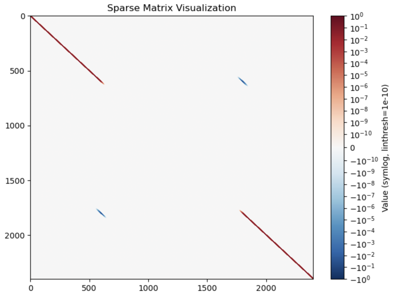
Side operator matrix
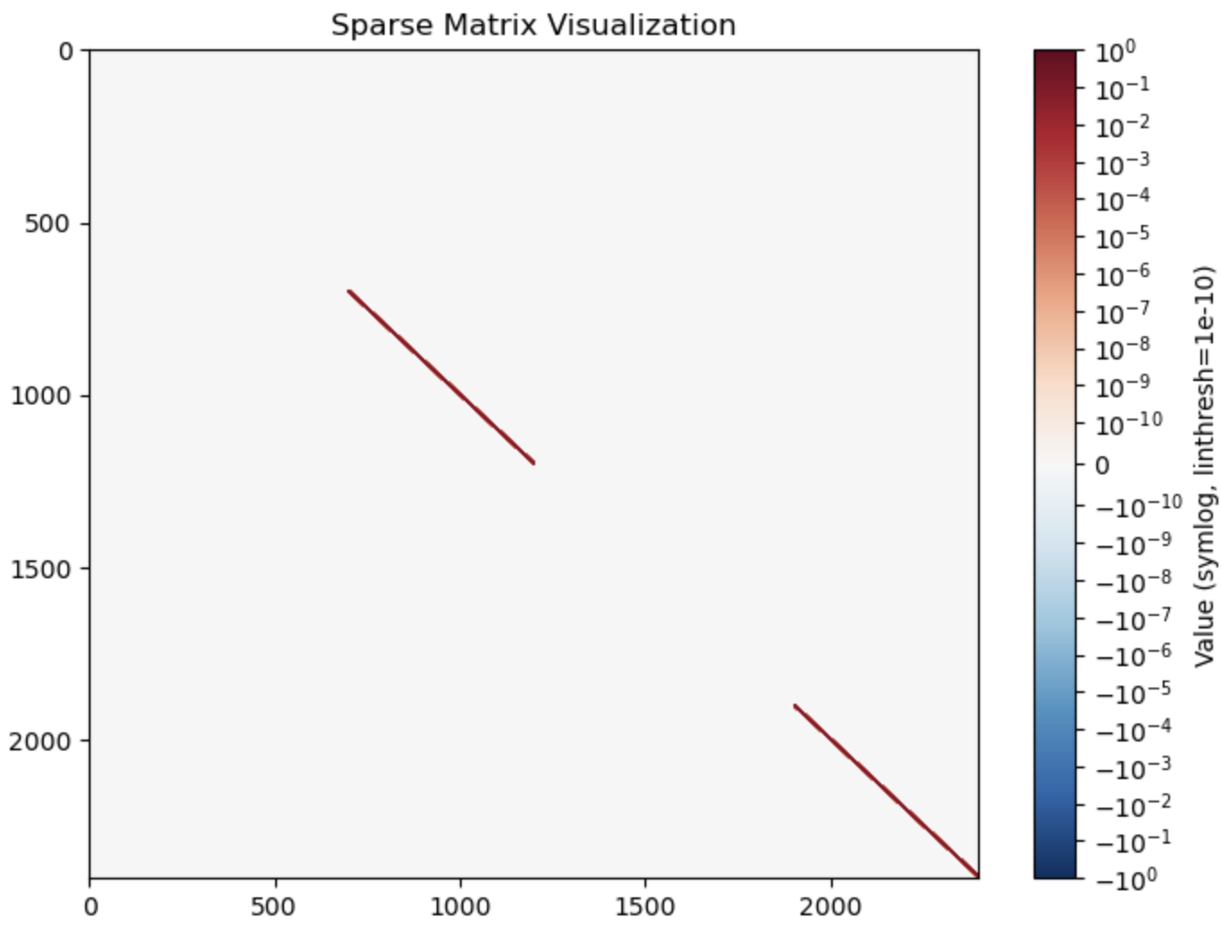
Side operator matrix. It is diagonal in the nuclear grid and repeated across electronic sectors. Entries switch from 0 to 1 across the selected dividing surface, so the heat map shows two diagonal active regions.

Flux operator

In the Heisenberg picture, \(h(t)=e^{iHt/\hbar}he^{-iHt/\hbar}\). Differentiating the two exponentials gives \(\dot h(t)=(i/\hbar)[H,h(t)]\). At \(t=0\), the rate of change of product-side occupancy is the flux operator:

\[ F=\frac{i}{\hbar}[H,h]. \]

Because \(h\) is a function of position, local potential terms commute with it. The visible structure mainly comes from \([T,h]\).
Flux operator matrix
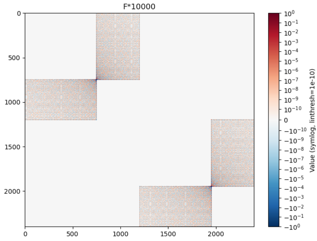
Flux matrix. Nonzero elements concentrate between grid points that lie on opposite sides of the dividing surface. The two electronic-state sectors repeat this pattern because the side operator does not distinguish electronic labels.

Thermalized flux

For Kubo-transformed rate formulas, a thermally dressed flux appears:
\[ F_{\mathrm{Kubo}}= \frac{1}{\beta}\int_0^\beta d\lambda\, e^{-(\beta-\lambda)H}F e^{-\lambda H}. \]
Thermalized flux matrix
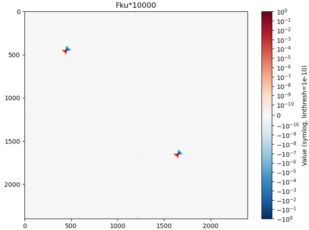
Thermalized flux matrix. The raw commutator structure is still visible, but imaginary-time Boltzmann factors suppress high-energy matrix components. This is why the matrix is more localized and lower amplitude than the bare flux matrix.

Time evolution and absorbing boundaries

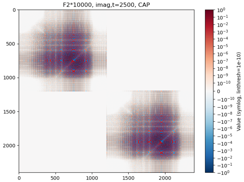
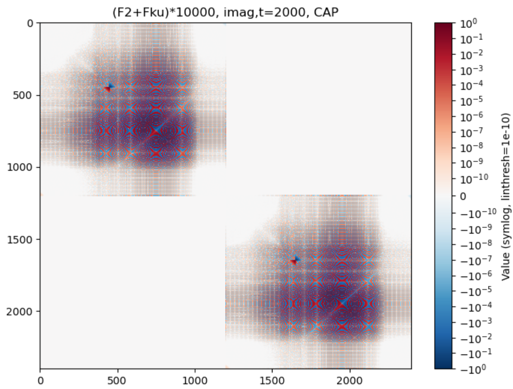
Finite DVR boxes reflect wavepackets unless the boundary is treated. A complex absorbing potential or mask damps boundary-region amplitude and reduces artificial recurrences.
Time-evolved flux-related matrix with CAP
Time-evolved flux-related matrix with a complex absorbing potential at \(t=2500\). Both axes are product-basis indices. Boundary-region matrix elements are damped, leaving compact interior structures.
Time-evolved flux-related matrix without CAP
The corresponding no-CAP case at the same time. Boundary-region structure remains stronger, which is the matrix-level sign of reflections in a finite simulation box.

These matrix pictures are the bridge between the method comparison in Part I and the concrete propagation in Part III. Once the block Hamiltonian is assembled, the wavepacket calculation is an application of the finite-dimensional unitary \(e^{-iHt/\hbar}\).

Code used in this note